

| << Chapter < Page | Chapter >> Page > |
Our first step was to generate a Y1 with random ones and zeros and see if there is any direct relationship to v1. The following demonstrates the code used to produce random binary values (impedances for Y1), while Fig 1 shows the output of the comparison.
for c = 1:m,
    if rand>0.5,
        y1(c) = one;else
        y1(c) = 0;end
endY1 = diag(y1);
v1 = nfc(Y1, S0);subplot(2,1,1)
stem(1:20, y1, 'r')title('Magnitude of Y1')

subplot(2,1,2)stem(1:20, abs(v1), 'b')
title('Magnitude of v1')
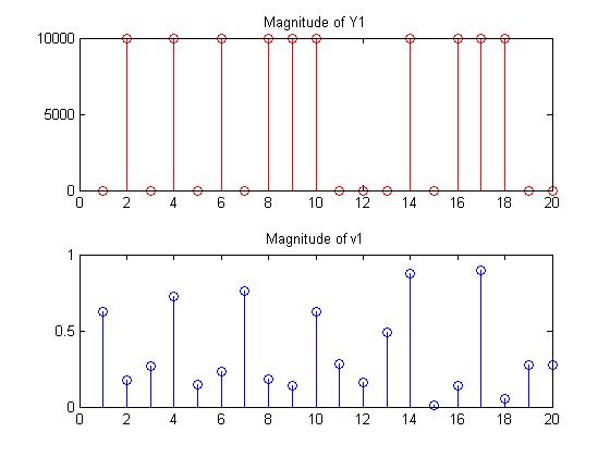
From these graphs, there was no obvious correlation between the “0’s” and “1’s” in Y1 and the values of v1. From here, a linear relationship was tested.
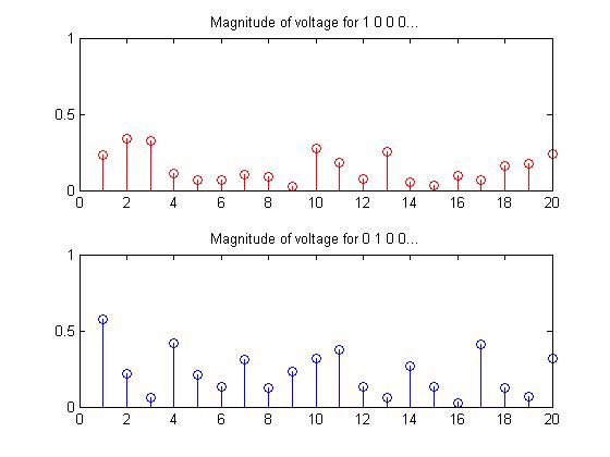
To determine if there was a linearity in computing the values of v1, we decided to compute the values of v1 for a Y1 matrix that had a diagonal of 11000000000000000000. As such, we first computed a set of v1 where there was a single 1 in the first port of Y1, and then a second set of v1 where there was a single 1 in the second port of Y1, and then added those two sets of values together. We were hoping to see if the result would produce a set of values of v1 that is identical to or similar to that which would be produced by a matrix with a diagonal of two 1's followed by 0's. The results of this test are shown in Fig 2 and Fig 3.
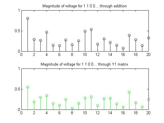
Looking at Fig 3. shows that the methods produce similar looking graphs, but each port has a slightly different magnitude. From these results we were able to conclude that the relationship between Y1 and v1 was non-linear.
Our next approach was to look at the Fourier transform of several different patterns, to see if a Fourier transform of the values of v1 could provide any insight into a relationship. The following set of graphs shows the values of the diagonal of the Y1 matrix, and the corresponding v1 values computed from it.
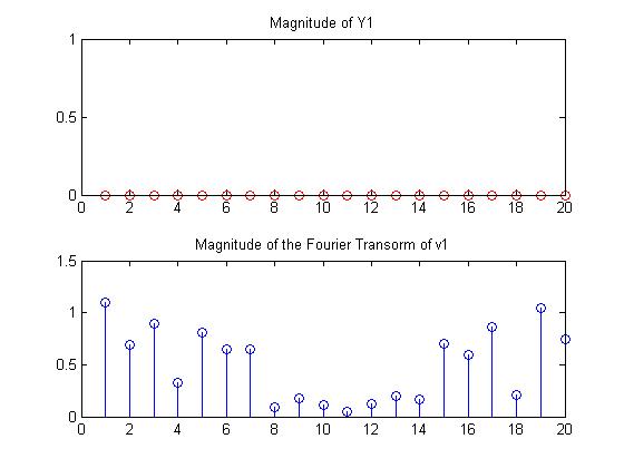


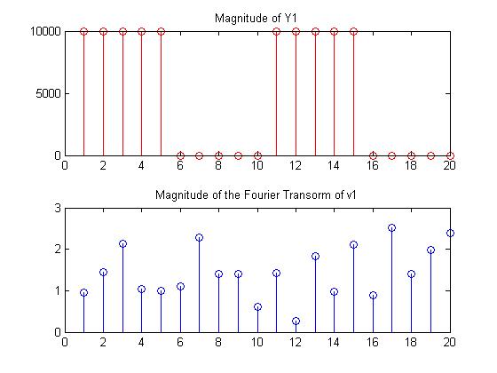
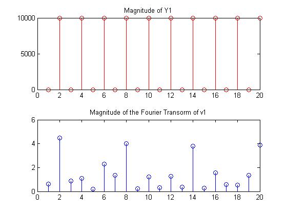

From these graphs, once again, there is no evidence that there is any relationship between any of the patterns and the values of v1, nor any relationship between Y1 and the Fourier transform of the values in v1.
Notification Switch
Would you like to follow the 'Near field communication simulation & Identification' conversation and receive update notifications?

|
|

|
|

|
|

|
|

|
|
|
|
|

|
|

|
|

|
|
|