0.3 Matched filter

Matched filtering

Matched filters underlie many signal classification systems in the real world, allowing systems to determine the likelihood of a signal being present in a noisy environment. They take the form a cross-correlation or convolution between the received signal and a desired signal, the presence (or absence) of which is to be ascertained. This cross-correlation may then be compared to a threshold, comprising a decision rule to test for the presence of the known signal.

Time-domain implementation

Within the time domain, matched filters take the form of a convolution of the received (x[n]) and desired (s[n]) signals.

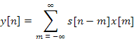
The output of this convolution will have a distinct peak when the reference and received signals are most closely correlated, and will have smaller fluctuations when they are uncorrelated or weakly correlated. Therefore, the time domain output of this convolution may simply be compared to a threshold. For samples where y[n] exceeds the threshold, we assume that x[n]contains our reference signal, and samples where y[n] falls below the threshold, x[n]does not contain our reference.

Frequency-domain implementation

Through the properties of the Fourier Transform, we can transform the above convolution into frequency-domain multiplication, giving rise to the frequency domain implementation of the matched filter.

While this implementation is obviously more computationally efficient if a frequency-domain copy of s[n] and x[n]already exists (as in the frequency-domain beamforming implementation), there is an obvious disadvantage for naïve implementations. If one simply took the DFT over all incoming samples to yield X[k], then no localization of the reference signal in time would be possible. That is, a decision could possibly be made about the existence or absence of the reference within the overall signal, but it could not be localized to a specific time within that interval.

The solution to this falls out of the Short Time Fourier Transform (STFT). If, instead of computing the DFT over all samples of the input, it is computed over a windowed subset, then we can still apply the above matched filter method while maintaining the ability to localize the signal’s occurrence in time. The new representation of this is as follows for non-time-varying s[n]:

The output of the frequency-domain matched filter can then be either transformed back into the time domain with the inverse STFT to be used with the existing per-sample decision rule, or can be used as the input to a frequency domain interpretation of the decision rule. The latter is obviously more computationally efficient, and is, at its simplest, the L ² norm of Y[k, t].

P[n] may then be compared to a threshold to determine the presence or absence of the reference signal within the STFT slice n.