0.2 Implementation

Implementation

Our implementation of the system was based around a controller program, which accepts the password to be transmitted, and then simulate the transmission and reconstruction. The program then returns whether or not the password received is the same as that which activated the system. In the final application, the controller is called repeatedly until the system is activated; it returns immediately after a non-match, and continues in sequence after the first element is matched.

For each of the passwords element’s iterations in the controller the following algorithm is used. The threshold is set to [the minimum value of the ideal signal minus three times the standard deviation of the base noise] (in our case one), and the mask is initialized to all ones. Then we prime the noise to reach either that standard deviation or less by priming the running total with a series of samples, the exact number of which is determined by the standard deviation of the noise. Then we execute the following function until either it runs a set number of times, or succeeds. Then the program compares the reconstructed signal after the iteration with the ideal signals, and returns if there is a reasonable match.

This function does the following four times: it samples the signal, updates the running total, and counts whether the maximum imaginary or real part of the Fourier transform of the signal is greater than the threshold. If at least two of the four cycles result in a value greater than the threshold, the mask’s value at that point is set to the previous value of the mask; otherwise, the mask’s value is set to zero. This allows a degree of leniency (which is useful in an inherently probabilistic method) and drastically reduces the probability of failure, albeit at the expense of increasing processing time.

The priming of the noise either reduces it to a standard deviation of two and a half, or three, based on the standard deviation of the noise. The method which is selected will result in fewer net samples required than the alternative method: although processing the information can take large quantities of samples, pre-processing requires sd^2/(2.5^2) or sd^2/(3^2) samples; hence, a larger denominator can cut off incredible quantities of samples. The reason why these values in particular were selected is that experimentally we determined that at 2.5 standard deviations, most signals required only one additional sample to become fully reconstructed, while at 3 standard deviations, they took a couple dozen to a few hundred, and a maximum of a few thousand additional samples, but it appeared to terminate the vast majority of the time as shown in Figure 1 and Figure 2.

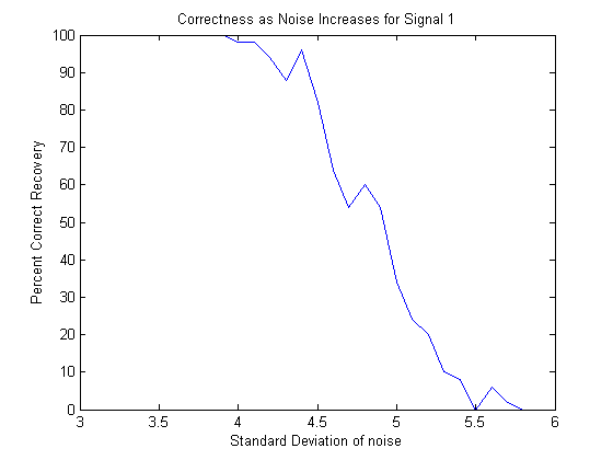
The success of a simple signal as a function of the standard deviation of the noise for a single cycle of a sinusoid with no priming(50 repetitions at each point).

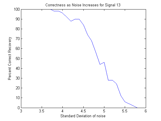
The success of a sum of a frequency one sine wave, a frequency four sine wave, and a frequency 20 cosine wave as a function of the standard deviation of the noise with no priming(50 repetitions at each point).

The priming is a necessity, since without it, the probability of success decreases rapidly as the standard deviation increases, but with it the probability of success, while not one, remains constantly above 99%. This is because after priming the effective standard deviation is always three or less, making the original signal consistently recoverable.

Timing analysis

All of the initializitions before the priming, assignations etc. require O(1) operations. The priming itself requires O(sd^2) operations. The post priming processing, requires O(library size) operations since although the fft is O(N*logN), N is bounded and therefore even if the sd wasn’t bounded to minimize the computation it still would always be less than a constant value. The only variable processing part is the comparisons with the library, which is O(libsize*N*logN) with N being bounded, simplifying to O(libsize). This means that the algorithm itself is O(sd^2)+O(libsize)=O(sd^2) since libsize will tend to be small. This is supported by experimental results as shown in Figure 1 and Figure 2.

The average time of execution as a function of the standard deviation of the noise for a single cycle sinusoid (50 repetitions per point).

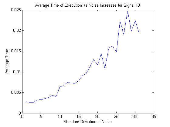
The average time of execution as a function of the standard deviation of the noise for the sum of a frequency 1, sine wave, a frequency 4 sine wave, and a frequency 20 cosine wave (50 repetitions per point).

For a real world application, it is also important to know not only the time it takes to execute the entire program, but also the number of samples that are required in order to reconstruct the signal. This is because the signal will only be transmitted for a limited time, so the hardware must be able to take the right number of samples in that time. From the processing perspective, even with very slow hardware the signal could eventually be reconstructed, but the same is not the case if the correct number of samples cannot be garnered. The number of samples required is always on O(sd^2) specifically sd^2/6.25+1 if sd<76, and sd^2/9+~200 if sd>=76. The experimental values are shown in Figure 3 and Figure 4.

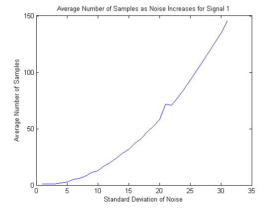
The average number of samples required to reconstruct the signal as standard deviation increases for a single cycle sine wave (50 repetitions at each point).

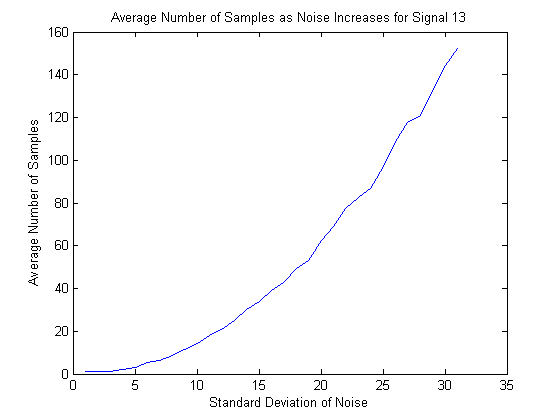
The average number of samples to reconstruct the signal as a function of the standard deviation of the noise for the sum of a frequency 1 sine wave, a frequency 4 sine wave, and a frequency 20 cosine wave (50 repetitions per point).

Examples of execution

All of the following figures are comprised of a series of graphs. The first graph is the initial signal with noise, as well as the initial signal; the next four graphs are the reconstructed signal at consecutive iterations along with the initial signal; the final graph is the final reconstructed signal along with the initial signal.

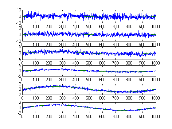
Execution from algorithm for signal 1, a frequency 1 sine wave with noise standard deviation of 5.

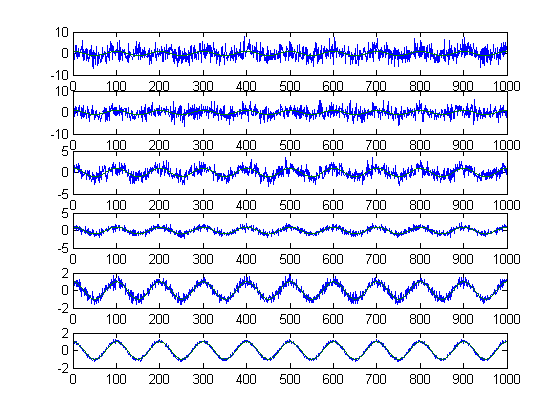
Execution from algorithm for signal 10, a frequency 10 cosine wave with noise standard deviation of 5.

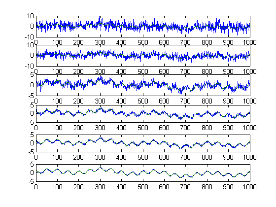
Execution from algorithm for signal 13, the sum of a frequency 1 sine wave, a frequency 4 sine wave, and a frequency 20 cosine wave with noise standard deviation of 5.