0.2 Derivation of the equations for a basic fdm-tdm transmux  (Page 4/10)

The computation of the $\left\{v\right(r,p\left)\right\}$ has several names in the literature. In some cases, it is referred to simply as the preprocessor or weighting processor. From the DFT-based filter bank interpretation of the transmultiplexer, in which the filter pulse function $h\left(k\right)$ is viewed as a spectral window function, the operation is called windowing and folding. Some of the first researchers in the area [link] termed it polyphase filtering . Even though the reasons for this name are fairly obscure, it is commonly used.

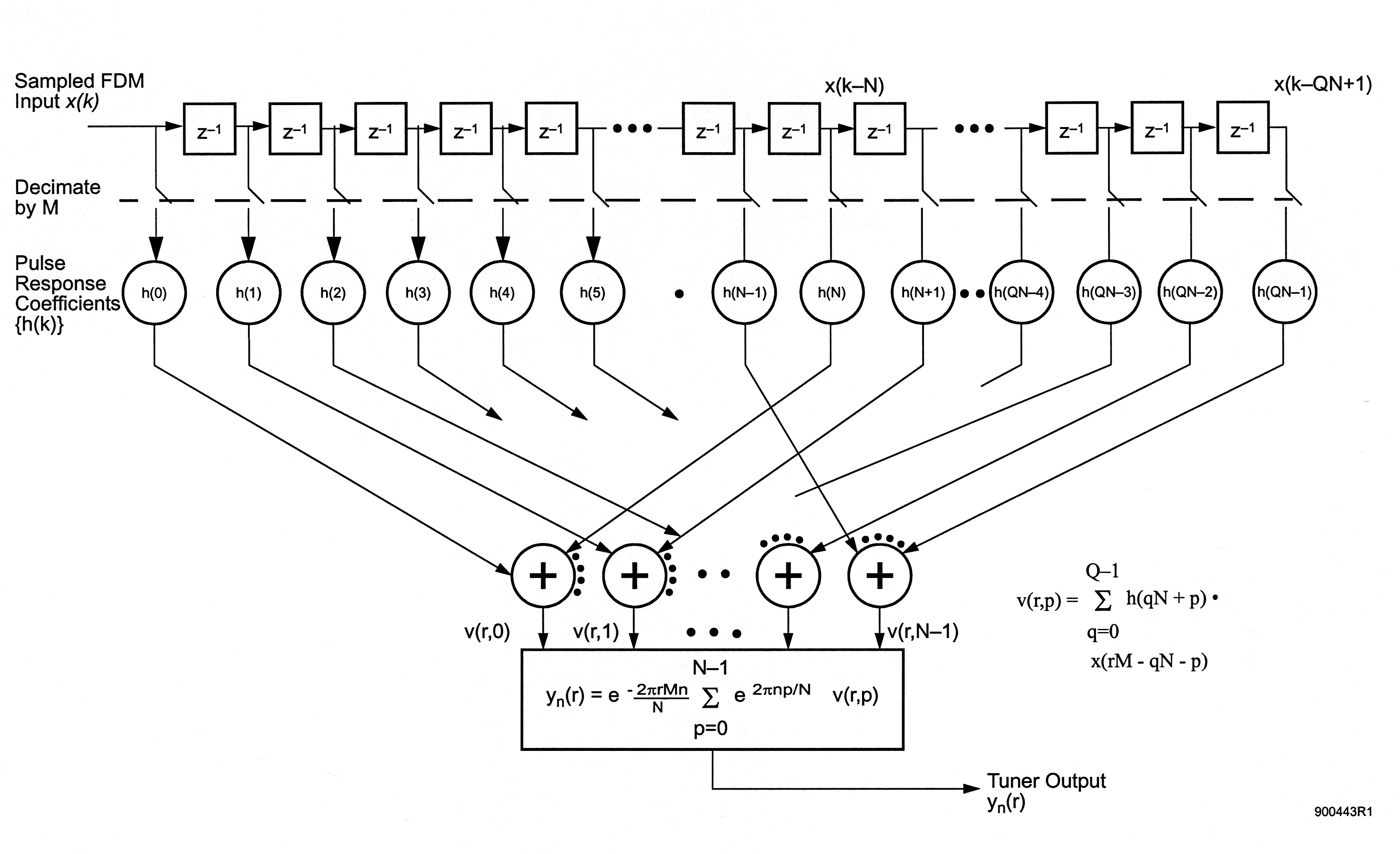
Once the input data has been preprocessed, windowed and folded, or polyphase filtered, as you will, the resulting N values of $v(r,p)$ are Fourier-transformed to produce $y_n\left(r\right)$ . Notice that all of this computation must be repeated for each value of r .

It will be useful later to know how much computation is required to implement this simplified tuner. Assume for this calculation that the input data $x\left(k\right)$ is complex-valued and that the pulse response $h\left(k\right)$ is real-valued. If so, then $2QN$ multiply-add operations are needed for each computation of the $\left\{v\right(r,p\left)\right\}$ and $4N$ multiply-adds (approximately) are needed for the computation of the single point of the DFT, all of this at the decimated sampling rate of $\frac{f_s}{M}$ . A conventional tuner using a real-valued, L-point pulse response and complex input data requires $4f_s$ multiply-adds for the mixer and $\frac{2f_{s}L}{M}$ multiply-adds for the filtering. Comparing the two shows that the filtering/weighting is exactly the same for the two, while the tuning vs. DFT comparison depends on the relative values of M and N . Using the example of the basic transmux , where $N=M$ , we find that the two are equal. When $M<N$ , the simplified equations actually require slightly more computation. Why then do we go to this trouble?

Generalization to the fft-based digital transmultiplexer

What if we desire to tune a second channel, say one that has a center frequency of $f_l=m·\Delta f$ ? Following through the derivation done before, we find that $y_m\left(r\right)$ is given by the same equations except that n is replaced with m . Examining the situation more closely we notice that the $\left\{v\right(r,p\left)\right\}$ need not be recomputed to obtain the second tuner output. In fact, the only operation required to obtain the second tuner output is to recompute the inverse DFT, but this time evaluated for the index m instead of n . The conventional tuning approach must be completely repeated to obtain the output for another channel. It is usually the case that the computation of the $\left\{v\right(r,p\left)\right\}$ is much larger than the computation required for the DFT. The fact that it need not be repeated quickly makes the preprocessor/DFT scheme significantly more efficient than the conventional digital tuner approach as the number of channels to be tuned grows. If we use the number of multiply-adds as an indication of computational complexity, and if we denote the number of channels to be tuned by the integer C , we can quantify this comparison by noting that

are needed for C conventional decimated digital tuners while