0.2 Cartesian vectors and tensors: their calculus  (Page 5/9)

since ${\overline{a}}_j=l_{ij}{a}_i$ so $\nabla \varphi$ is a vector.

The unit vector in the direction of $d\mathbf{x}$ is $\mathbf{u}=d\mathbf{x}/ds$ . The derivative of $\varphi$ in the direction of $\mathbf{u}$ is

If $\varphi \left(x\right)=c$ is a surface, then $\nabla \varphi$ is normal to the surface. To prove this, let $d\mathbf{x}$ be a differential distance on the surface. The differential of $\varphi$ along $d\mathbf{x}$ is zero for any $d\mathbf{x}$ on the surface. This implies that the scalar product of $\nabla \varphi$ with any vector on the surface is zero or that $\nabla \varphi$ has zero component or projection on the tangent plane and thus $\nabla \varphi$ is normal to the surface. Also, since $\nabla \varphi$ is normal to the surface, the derivative of $\varphi$ is a maximum in the direction normal to the surface.

The divergence of a vector field

The symbolic scalar or dot product of the operator $\nabla$ and a vector is called the divergence of the vector field. Thus for any differentiable vector field $\mathbf{a}\left(\mathbf{x}\right)$ we write

The divergence is a scalar because it is the scalar product and because it is the contraction of the second order tensor $a_{i,j}$ .

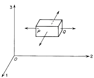
We will now demonstrate why the $\nabla •$ operation on a vector field is called the divergence. Suppose that an elementary parallelepiped is set up with one corner $P$ at $x_1,x_2,x_3$ and the diagonally opposite one $Q$ at $x_1+d{x}_1$ , $x_2+d{x}_2$ , $x_3+d{x}_3$ as shown in Fig. 3.7. The outward unit normal to the face through $Q$ which is perpendicular to $\mathit{01}$ is ${\mathbf{e}}_{\left(1\right)}$ , whereas the outward normal to the parallel face through $P$ is $-{\mathbf{e}}_{\left(1\right)}$ . Suppose $\mathbf{a}\left(\mathbf{x}\right)$ is a differentiable flux vector field. We are going to compute the net flux of $\mathbf{a}$ across the bounding surfaces of the parallelepiped. The value of the normal component of $\mathbf{a}$ at some point on the two faces perpendicular to the 01 direction are

Thus if $\mathbf{n}$ denotes the outward normal and $dS$ is the area $d{x}_{2}d{x}_3$ of these two faces, we have a contribution from them to the surface integral $\underset{S}{\int \int ◯}\mathbf{a}\mathbf{n}dS$ of

where $O\left(d{x}^4\right)$ denotes terms proportional to fourth power of $dx$ . Similar terms with $\delta a_2/\delta x_2$ and $\delta a_3/\delta x_3$ will be given by contributions of the other faces so that for the whole parallelepiped whose volume $dV=d{x}_{1}d{x}_{2}d{x}_3$ we have

If we let the volume shrink to zero we have

If $\mathbf{a}$ is a flux, then the surface integral is the net flux of $\mathbf{a}$ out of the volume. In particular, let $\mathbf{a}$ be the fluid velocity, which can be thought as a volumetric flux. Then the divergence of velocity is the volumetric expansion per unit volume. A vector field with identically zero divergence is called solenoidal . An incompressible fluid has a solenoidal velocity field. If the flux field of a certain property is solenoidal there is no generation of that property within the field, for all that flows into an infinitesimal element flows out again.

If $\mathbf{a}$ is the gradient of a scalar function $\nabla \varphi$ , its divergence is called the Laplacian of $\varphi$ .

A function that satisfies Laplace's equation ${\nabla }^2\varphi =0$ is called a potential function or a harmonic function . An irrotational, incompressible flow field has a velocity that is the gradient of a flow potential. Also, the steady-state temperature field in a homogeneous solid and the steady state pressure distribution of a single fluid phase flowing in porous media are solutions of Laplace's equation. In two dimensions the solutions of Laplace's equation can be found through the use of complex variables.