0.17 18. multiple regression: assumptions  (Page 2/2)

Have your data set open in SPSS. In this dataset, we will determine what variables, if any, are predictive of students’ Wechsler Full Scale IQ 3 (wifsiq). The 10 variables that we will use are: Picture Completion (pc), Information (inf), Coding (cod), Similarities (sim), Picture Arrangement (pa), Arithmetic (ari), Block Design (bd), Vocabulary (voc), Object Assembly (oa), and Comprehension (comp).

As with every statistical procedure, we need to check the underlying assumptions. One assumption involves the data being normally distributed. To check this assumption, we recommend that you calculate the standardized skewness coefficients and the standardized kurtosis coefficients, as discussed in other chapters.

* Skewness [Note. Skewness refers to the extent to which the data are normally distributed around the mean. Skewed data involve having either mostly high scores with a few low ones or having mostly low scores with a few high ones.] Readers are referred to the following sources for a more detailed definition of skewness: (External Link)&term_id=356 and (External Link)

To standardize the skewness value so that its value can be constant across datasets and across studies, the following calculation must be made: Take the skewness value from the SPSS output and divide it by the Std. error of skewness. If the resulting calculation is within -3 to +3, then the skewness of the dataset is within the range of normality (Onwuegbuzie&Daniel, 2002). If the resulting calculation is outside of this +/-3 range, the dataset is not normally distributed.

* Kurtosis [Note. Kurtosis also refers to the extent to which the data are normally distributed around the mean. This time, the data are piled up higher than normal around the mean or piled up higher than normal at the ends of the distribution.] Readers are referred to the following sources for a more detailed definition of kurtosis: (External Link)&term_id=326 and (External Link)

To standardize the kurtosis value so that its value can be constant across datasets and across studies, the following calculation must be made: Take the kurtosis value from the SPSS output and divide it by the Std. error of kurtosis. If the resulting calculation is within -3 to +3, then the kurtosis of the dataset is within the range of normality (Onwuegbuzie&Daniel, 2002). If the resulting calculation is outside of this +/-3 range, the dataset is not normally distributed.

Now that you have verified that your data are normally distributed, the extent to which linearity is present between each of the 10 independent variables listed above and the dependent variable of Full Scale IQ must be determined. For linearity, we will have SPSS conduct scatterplots for each IV and DV pair.

√ Graphs

√ Legacy Dialogs

√ Scatter/Dot

After clicking on Scatter/Dot, the following screen will appear. The Simple Scatter icon should be highlighted. If not, click on it.

√ Click on Define

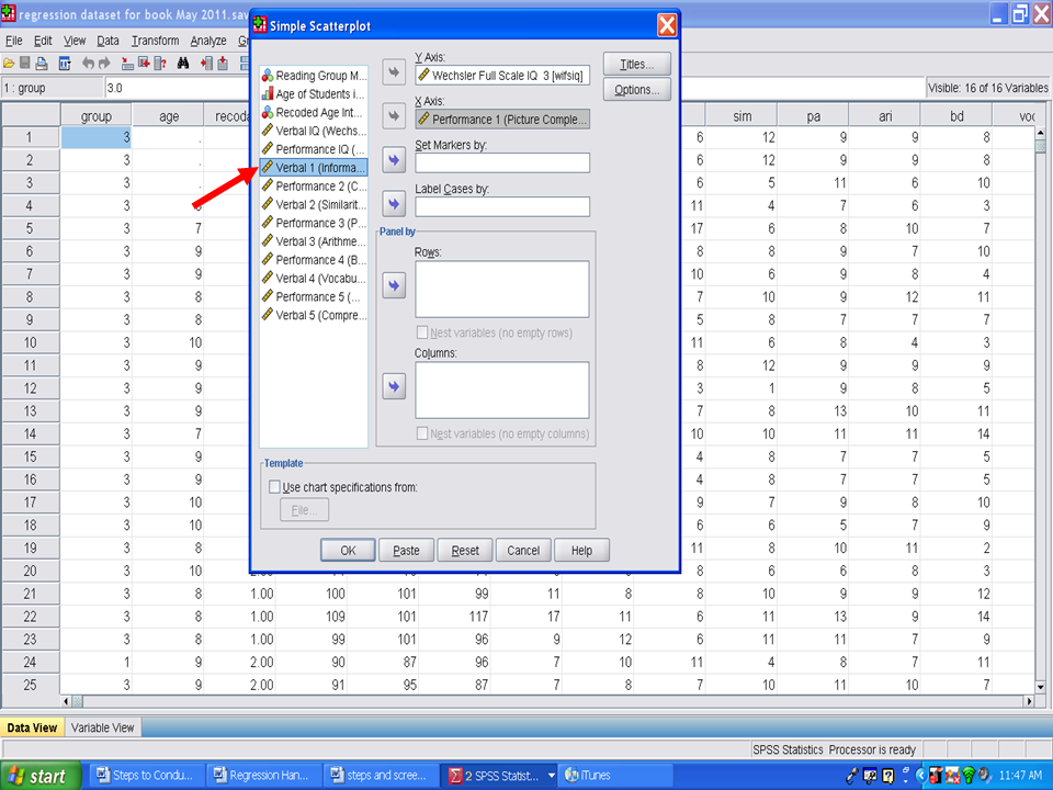
The following screen should now be present.

√ Drag one of the two variables of interest to the first box (Y axis) on the right hand side and the other variable of interest to the second box (X axis) on the right hand side. It does not matter which variable goes in the X or Y axis because your scatterplot results will be the same. For our purposes, we will place the variable we are trying to predict, Wechsler Full Scale IQ 3, in the Y Axis box and one of the variables (i.e., Performance 1) we will use to try to predict it.

√ Once you have a variable in each of the first two boxes, click on the OK tab on the bottom left hand corner of the screen.

√ Look at the scatterplot to determine whether a linear relationship is present. In the screenshot below, the relationship is very clearly linear.

You will need to repeat this process, for this example, nine more times. Leave the dependent variable of Wechsler Full Scale IQ 3 in the Y Axis box and replace the variable in the X Axis box with the next variable (i.e., Verbal 1). Then click on OK.

After you have verified that linearity is present for each independent variable with the dependent variable, we will examine the extent to which multicollinearity is not present. Multicollinearity refers to having variables that are highly correlated with each other. When variables are highly correlated in a multiple regression analysis, the unique contribution of each variable in predicting the dependent variable is difficult to determine. The reason for this difficulty is that highly interrelated variables are being used to predict the same variance in the dependent variable. Researchers/statisticians disagree on the specific correlation value that must be present for multicollinearity to exist. Some persons contend that correlations above .70 are necessary whereas other persons contend that the correlations must be above .90 for multicollinearity to exist.

If multicollinearity is present, you can leave it as it is, and have SPSS calculate the multiple regression. Multicollinearity influences the results regarding each predictor’s unique contribution. If your interest is in the overall or combined effect of the statistically significant predictors, then multicollinearity is not an issue. Other choices would be to remove one or more of the highly correlated variables from the regression analysis or to create an aggregate or composite of the highly correlated variables.

The choice that we recommend is to have SPSS calculate multicollinearity when the multiple regression analysis is calculated. More on this later.