<< Chapter < Page Chapter >> Page >
This module is the complementary teacher's guide for the "F Distribution and ANOVA" chapter of the Collaborative Statistics collection (col10522) by Barbara Illowsky and Susan Dean.
The F size 12{F} {} distribution is named after Ronald Fisher. Fisher is one of the most respected statisticians of all time. He did a lot of statistical work in biology and genetics and became chair of genetics at Cambridge University in England in 1949. In 1952, he was awarded knighthood.

This section is a very brief overview of the F size 12{F} {} distribution and two of its applications - One Way Analysis of Variance (ANOVA) and test of two variances. There are college courses which deal exclusively with these topics. ANOVA, particularly, is used regularly in industry.

    Explanation of sum of squares, mean square, and the f ratio for anova

  • k size 12{k} {} = the number of different groups
  • n j size 12{n rSub { size 8{j} } } {} = the size of the jth size 12{ ital "jth"} {} group
  • s j size 12{s rSub { size 8{j} } } {} = the sum of the values in the jth size 12{ ital "jth"} {} group
  • N size 12{N} {} = the total number of all the values combined
  • Total sample size: n j size 12{ Sum {n rSub { size 8{j} } } } {}
  • x = one value: x = s j size 12{ Sum {x} = Sum {s rSub { size 8{j} } } } {}
  • Sum of squares of all values from every group combined: x 2 size 12{ Sum {x rSup { size 8{2} } } ={}} {}
  • Between group variability: SS total = x 2 x 2 N size 12{ ital "SS" rSub { size 8{ ital "total"} } = Sum {x rSup { size 8{2} } } - { { left ( Sum {x} right ) rSup { size 8{2} } } over {N} } } {}
  • Total sum of squares: x 2 ( x ) 2 N size 12{ Sum {x rSup { size 8{2} } } - { { \( Sum {x} \) rSup { size 8{2} } } over {N} } } {}
  • Explained variation- sum of squares representing variation among the different samples SS between = [ ( sj ) 2 n j ] ( s j ) 2 N size 12{ ital "SS" rSub { size 8{ ital "between"} } = Sum { \[ { { \( ital "sj" \) rSup { size 8{2} } } over {n rSub { size 8{j} } } } \] } - { { \( Sum {s rSub { size 8{j} } \) rSup { size 8{2} } } } over {N} } } {}
  • Unexplained variation- sum of squares representing variation within samples due to chance: SS within = SS total SS between size 12{ ital "SS" rSub { size 8{ ital "within"} } = ital "SS" rSub { size 8{ ital "total"} } - ital "SS" rSub { size 8{ ital "between"} } } {}
  • df's for different groups (df's for the numerator): df between = k 1 size 12{ ital "df" rSub { size 8{ ital "between"} } =k - 1} {}
  • Equation for errors within samples (df's for the denominator): df within = N k size 12{ ital "df" rSub { size 8{ ital "within"} } =N - k} {}
  • Mean square (variance estimate) explained by the different groups: MS between = SS between df between size 12{ ital "MS" rSub { size 8{ ital "between"} } = { { ital "SS" rSub { size 8{ ital "between"} } } over { ital "df" rSub { size 8{ ital "between"} } } } } {}
  • Mean square (variance estimate) that is due to chance (unexplained): MS within = SS within df within size 12{ ital "MS" rSub { size 8{ ital "within"} } = { { ital "SS" rSub { size 8{ ital "within"} } } over { ital "df" rSub { size 8{ ital "within"} } } } } {}
  • F ratio or F statistic of two estimates of variance: F = MS between MS within size 12{F= { { ital "MS" rSub { size 8{ ital "between"} } } over { ital "MS" rSub { size 8{ ital "within"} } } } } {}
The above calculations were done with groups of different sizes. If the groups are the same size, the calculations simplify somewhat and the F ratio can be written as:

F ratio formula

F = n ( s x ) 2 ( s pooled ) 2 size 12{F= { {n cdot \( s rSub { size 8{ - x} } \) rSup { size 8{2} } } over { \( s rSub { size 8{ ital "pooled"} } \) rSup { size 8{2} } } } } {}

    Where...

  • ( s x ) 2 = size 12{ \( s rSub { size 8{ - x} } \) rSup { size 8{2} } ={}} {} the variance of the sample means
  • n = size 12{n={}} {} the sample size of each group
  • ( s pooled ) 2 = size 12{ \( s rSub { size 8{ ital "pooled"} } \) rSup { size 8{2} } ={}} {} the mean of the sample variances (pooled variance)
  • df numerator = k 1 size 12{ ital "df" rSub { size 8{ ital "numerator"} } =k - 1} {}
  • df denominator = k ( n 1 ) = N k size 12{ ital "df" rSub { size 8{ ital "denominator"={}} } k \( n - 1 \) =N - k} {}

These calculations are easily done with a graphing calculator or a computer program. We present the information in the chapter assuming some kind of technology will be used.

For ANOVA, the samples must come from normally distributed populations with the same variance, and the samples must be independent. The ANOVA test is right-tailed.

In a test of two variances, the samples must come from normal populations and must be independent of each other.

(one-way anova)

Three different diet plans are to be tested for average weight loss. For each diet plan, 4 dieters are selected and their weight loss (in pounds) in one month's time is recorded.

Plan 1 Plan 2 Plan 3
5 3.5 8
4.5 7 4
4 6 3.5
3 4 4.5

Is the average weight loss the same for each plan? Conduct an ANOVA test with a 1% level of significance.

Let μ 1 size 12{μ rSub { size 8{1} } } {} , μ 2 size 12{μ rSub { size 8{2} } } {} , and μ 3 size 12{μ rSub { size 8{3} } } {} be the population means for the three diet plans.

  • H o : μ 1 = μ 2 = μ 3 size 12{H rSub { size 8{o} } :μ rSub { size 8{1} } =μ rSub { size 8{2} } =μ rSub { size 8{3} } } {}
  • H a : size 12{H rSub { size 8{a} } :} {} Not all pairs of means are equal.
  • df numerator = 3 1 = 2 size 12{ ital "df" rSub { size 8{ ital "numerator"} } =3 - 1=2} {}
  • df deno min ator = 12 3 = 9 size 12{ ital "df" rSub { size 8{ ital "deno""min" ital "ator"} } ="12" - 3=9} {}

The distribution for the test is F 2,9 size 12{F rSub { size 8{2,9} } } {}

Using a calculator or computer, the test statistic is F = 0 . 47 size 12{F=0 "." "47"} {} . The notation used for the F size 12{F} {} statistic may also be F ' size 12{F'} {} or F 2,9 size 12{F rSub { size 8{2,9} } } {} (like the distribution). The TI-83/84 series has the function ANOVA in STAT TESTS. Enter the lists of data separated by commas.

If you use the formulas for groups of the same size, the calculations are as follows:

Sample means are 4.13, 5.13, and 5, respectively. Sample standard deviations are 0.8539, 1.6250, and 2.0412, respectively.

( s x ) 2 = 0 . 2956 size 12{ \( s rSub { size 8{ - x} } \) rSup { size 8{2} } =0 "." "2956"} {} The variance of the sample means
( s pooled ) 2 = 2 . 5416 size 12{ \( s rSub { size 8{ ital "pooled"} } \) rSup { size 8{2} } =2 "." "5416"} {} The mean of the sample variances
n = 4 size 12{n=4} {} The sample size of each group
F = 4 0 . 2956 2 . 5416 size 12{F= { {4 cdot 0 "." "2956"} over {2 "." "5416"} } } {}

Probability Statement:
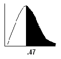
 P ( F > 0 . 47 ) = 0 . 6395 size 12{P \( F>0 "." "47" \) =0 "." "6395"} {}

Probability graph showing the all values greater than .47 shaded
p size 12{p} {} -value = 0 . 6395 size 12{ {}=0 "." "6395"} {}

Since α < p size 12{a<p} {} -value, do not reject H o size 12{H rSub { size 8{o} } } {} .

There is not sufficient evidence to conclude that the three diet plans are different. It appears that the three diet plans work equally well. The average weight loss is the same for all three plans.

(test of two variances):

Machine A makes a box and machine B makes a lid. For the lid to fit the box correctly, the variances should be nearly the same. There is a suspicion that the variance of the box is greater than the variance of the lid. The following data was collected.

Machine A (Box) Machine B (Lid)
Number of Parts 9 11
Variance 150 45

Are the machines working properly? Test at a 5% level of significance.

Let σ A 2 size 12{σ rSub { size 8{A rSup { size 6{2} } } } } {} and σ B 2 size 12{σ rSub { size 8{B rSup { size 6{2} } } } } {} be the population variances for machine A and machine B, respectively

  • H o : σ A 2 = σ B 2 size 12{H rSub { size 8{o} } :σ rSub { size 8{A rSup { size 6{2} } } } =σ rSub {B rSup { size 6{2} } } } {}
  • H a : σ A 2 > σ B 2 size 12{H rSub { size 8{a} } :σ rSub { size 8{A rSup { size 6{2} } } }>σ rSub {B rSup { size 6{2} } } } {}
  • n A = 9 size 12{n rSub { size 8{A} } =9} {}
  • n B = 11 size 12{n rSub { size 8{B} } ="11"} {}
  • df numerator = 9 1 size 12{ ital "df" rSub { size 8{ ital "numerator"} } =9 - 1} {}
  • df deno min ator = 11 1 = 10 size 12{ ital "df" rSub { size 8{ ital "deno""min" ital "ator"} } ="11" - 1="10"} {}

The distribution for the hypothesis test is F 8, 10 size 12{F rSub { size 8{8,"10"} } } {}

If you are using the TI-83/84 calculators, use the function 2-SAMPFTest for the test.

Using the formulas,

The test statistic is F = [ ( s A ) 2 ( σ A ) 2 ] [ ( s B ) 2 ( σ B ) 2 ] = size 12{F= { { \[ { { \( s rSub { size 8{A} } \) rSup { size 8{2} } } over { \( σ rSub { size 8{A} } \) rSup { size 8{2} } } } \] } over { \[ { { \( s rSub { size 8{B} } \) rSup { size 8{2} } } over { \( σ rSub { size 8{B} } \) rSup { size 8{2} } } } \]} } ={}} {}

( s A ) 2 ( s B ) 2 = 150 45 = 3 . 3 3 ¯ size 12{ { { \( s rSub { size 8{A} } \) rSup { size 8{2} } } over { \( s rSub { size 8{B} } \) rSup { size 8{2} } } } = { {"150"} over {"45"} } =3 "." 3 {overline {3}} } {}

Since α > p size 12{a>p} {} -value, reject the null hypothesis.

There is sufficient evidence to conclude that the box and lid do not fit each other. The variance of the box is larger.

Assign practice

Have the students work collaboratively to complete the Practice .

Assign homework

Assign Homework . Suggested homework: 1, 3, 4, 5.

Questions & Answers

differentiate between demand and supply giving examples
Lambiv Reply
differentiated between demand and supply using examples
Lambiv
what is labour ?
Lambiv
how will I do?
Venny Reply
how is the graph works?I don't fully understand
Rezat Reply
information
Eliyee
devaluation
Eliyee
t
WARKISA
hi guys good evening to all
Lambiv
multiple choice question
Aster Reply
appreciation
Eliyee
explain perfect market
Lindiwe Reply
In economics, a perfect market refers to a theoretical construct where all participants have perfect information, goods are homogenous, there are no barriers to entry or exit, and prices are determined solely by supply and demand. It's an idealized model used for analysis,
Ezea
What is ceteris paribus?
Shukri Reply
other things being equal
AI-Robot
When MP₁ becomes negative, TP start to decline. Extuples Suppose that the short-run production function of certain cut-flower firm is given by: Q=4KL-0.6K2 - 0.112 • Where is quantity of cut flower produced, I is labour input and K is fixed capital input (K-5). Determine the average product of lab
Kelo
Extuples Suppose that the short-run production function of certain cut-flower firm is given by: Q=4KL-0.6K2 - 0.112 • Where is quantity of cut flower produced, I is labour input and K is fixed capital input (K-5). Determine the average product of labour (APL) and marginal product of labour (MPL)
Kelo
yes,thank you
Shukri
Can I ask you other question?
Shukri
what is monopoly mean?
Habtamu Reply
What is different between quantity demand and demand?
Shukri Reply
Quantity demanded refers to the specific amount of a good or service that consumers are willing and able to purchase at a give price and within a specific time period. Demand, on the other hand, is a broader concept that encompasses the entire relationship between price and quantity demanded
Ezea
ok
Shukri
how do you save a country economic situation when it's falling apart
Lilia Reply
what is the difference between economic growth and development
Fiker Reply
Economic growth as an increase in the production and consumption of goods and services within an economy.but Economic development as a broader concept that encompasses not only economic growth but also social & human well being.
Shukri
production function means
Jabir
What do you think is more important to focus on when considering inequality ?
Abdisa Reply
any question about economics?
Awais Reply
sir...I just want to ask one question... Define the term contract curve? if you are free please help me to find this answer 🙏
Asui
it is a curve that we get after connecting the pareto optimal combinations of two consumers after their mutually beneficial trade offs
Awais
thank you so much 👍 sir
Asui
In economics, the contract curve refers to the set of points in an Edgeworth box diagram where both parties involved in a trade cannot be made better off without making one of them worse off. It represents the Pareto efficient allocations of goods between two individuals or entities, where neither p
Cornelius
In economics, the contract curve refers to the set of points in an Edgeworth box diagram where both parties involved in a trade cannot be made better off without making one of them worse off. It represents the Pareto efficient allocations of goods between two individuals or entities,
Cornelius
Suppose a consumer consuming two commodities X and Y has The following utility function u=X0.4 Y0.6. If the price of the X and Y are 2 and 3 respectively and income Constraint is birr 50. A,Calculate quantities of x and y which maximize utility. B,Calculate value of Lagrange multiplier. C,Calculate quantities of X and Y consumed with a given price. D,alculate optimum level of output .
Feyisa Reply
Answer
Feyisa
c
Jabir
the market for lemon has 10 potential consumers, each having an individual demand curve p=101-10Qi, where p is price in dollar's per cup and Qi is the number of cups demanded per week by the i th consumer.Find the market demand curve using algebra. Draw an individual demand curve and the market dema
Gsbwnw Reply
suppose the production function is given by ( L, K)=L¼K¾.assuming capital is fixed find APL and MPL. consider the following short run production function:Q=6L²-0.4L³ a) find the value of L that maximizes output b)find the value of L that maximizes marginal product
Abdureman
types of unemployment
Yomi Reply
What is the difference between perfect competition and monopolistic competition?
Mohammed
Got questions? Join the online conversation and get instant answers!
Jobilize.com Reply

Get Jobilize Job Search Mobile App in your pocket Now!

Get it on Google Play Download on the App Store Now


Source:  OpenStax, Collaborative statistics teacher's guide. OpenStax CNX. Oct 01, 2008 Download for free at http://cnx.org/content/col10547/1.5
Google Play and the Google Play logo are trademarks of Google Inc.

Notification Switch

Would you like to follow the 'Collaborative statistics teacher's guide' conversation and receive update notifications?

Ask