The default settings in
dae.m are used to perform the
equalizer designs for three channels.The source alphabet is a binary
signal.
Each channel has a FIR impulse response, and its outputis summed with a sinusoidal interference and some uniform
white noise before reaching the receiver.The user is prompted for
choice of channels (0, 1, or 2),
maximum delay of the equalizer,
number of samples of training data,
gain of the sinusoidal interferer,
frequency of the sinusoidal interferer (in radians), and
magnitude of the white noise.
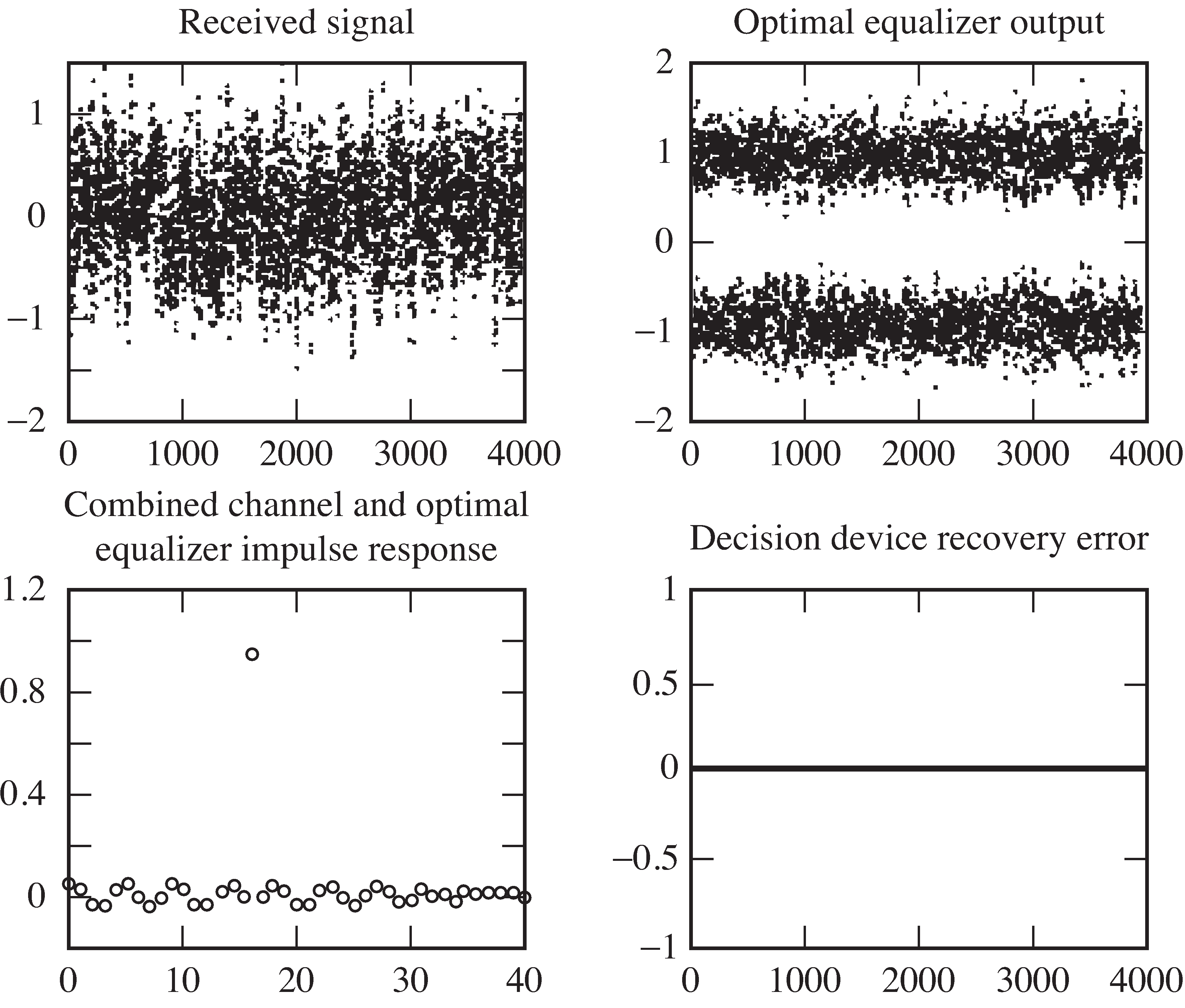
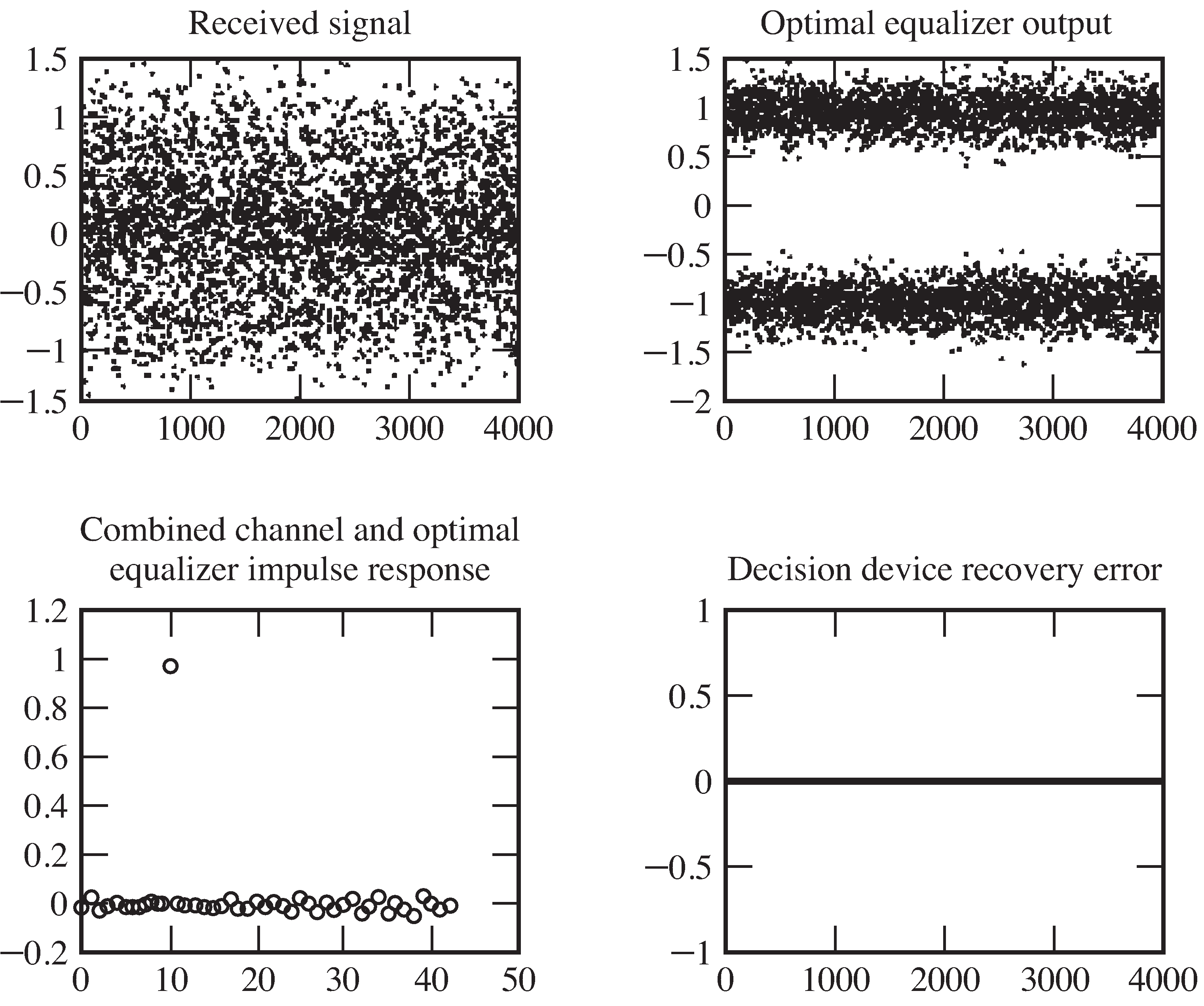
The program returns plots of the
received signal,
optimal equalizer output,
impulse response of the optimal equalizer and the channel,
recovery error at the output of the decision device,
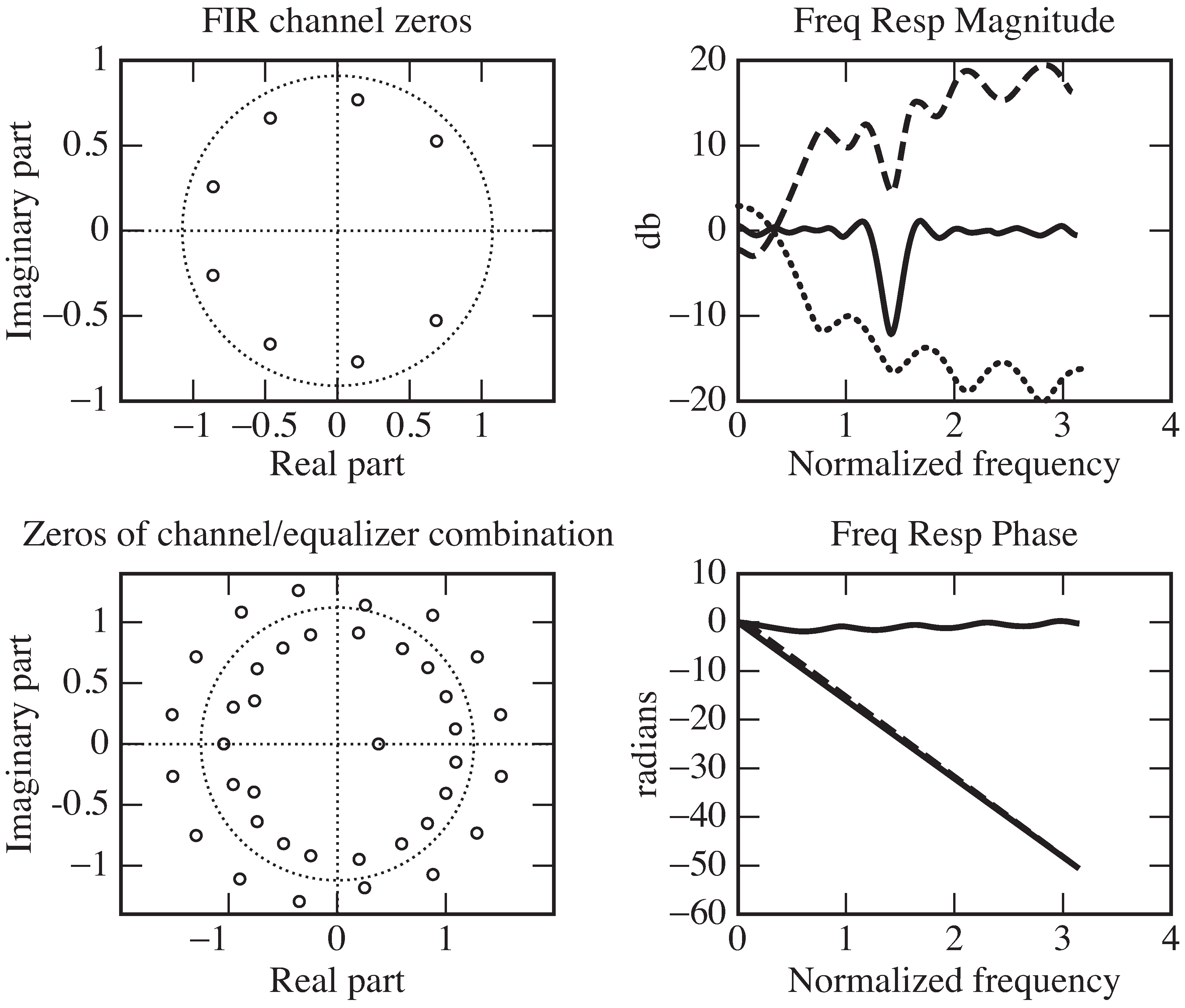
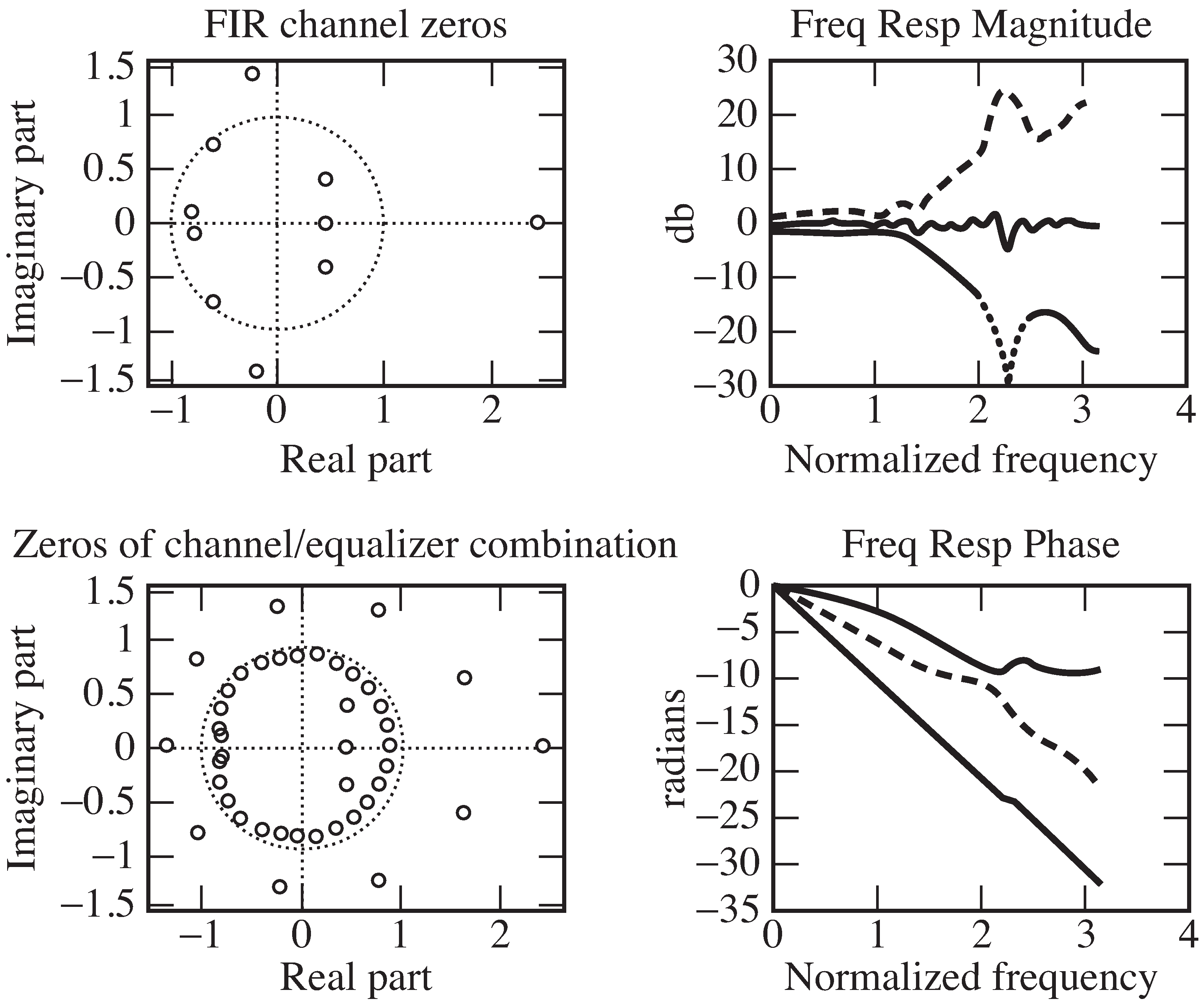
zeros of the channel and the combined channel–equalizer pair, and
magnitude and phase frequency responses of the
channel, equalizer, and the combined channel–equalizer pair.
For the default channels and values,
these plots are shown in
[link] –
[link] .
The program also prints the condition number of
, the minimum average squared recovery error
(i.e., the minimum value achieved by the performance functionby the optimal equalizer for the optimum delay
),
the optimal value of the delay
,
and the percentage of decision device output errors inmatching the delayed source.
These values were as follows:
Channel 0
condition number: 130.2631
minimum value of performance function: 0.0534
optimum delay: 16
percentage of errors: 0
Trained least-squares equalizer for Channel 0: Time responses.
The received signal is messy and cannot be used directly torecover the message. After passing through the optimal equalizer,
there is sufficient separation to open the eye.The bottom left figure shows the impulse response of the
channel convolved with the impulse response of the optimalequalizer, it is close to an ideal response (which would be one
at one delay and zero everywhere else). The bottom right plotshows that the message signal is recovered without error.Trained least-squares equalizer for Channel 0: Singularities
and frequency responses. The large circles show the locations of thezeros of the channel in the upper left plot and the locations of the
zeros of the combined channel–equalizer pair in the lower left.The *** represents the frequency response of the channel,
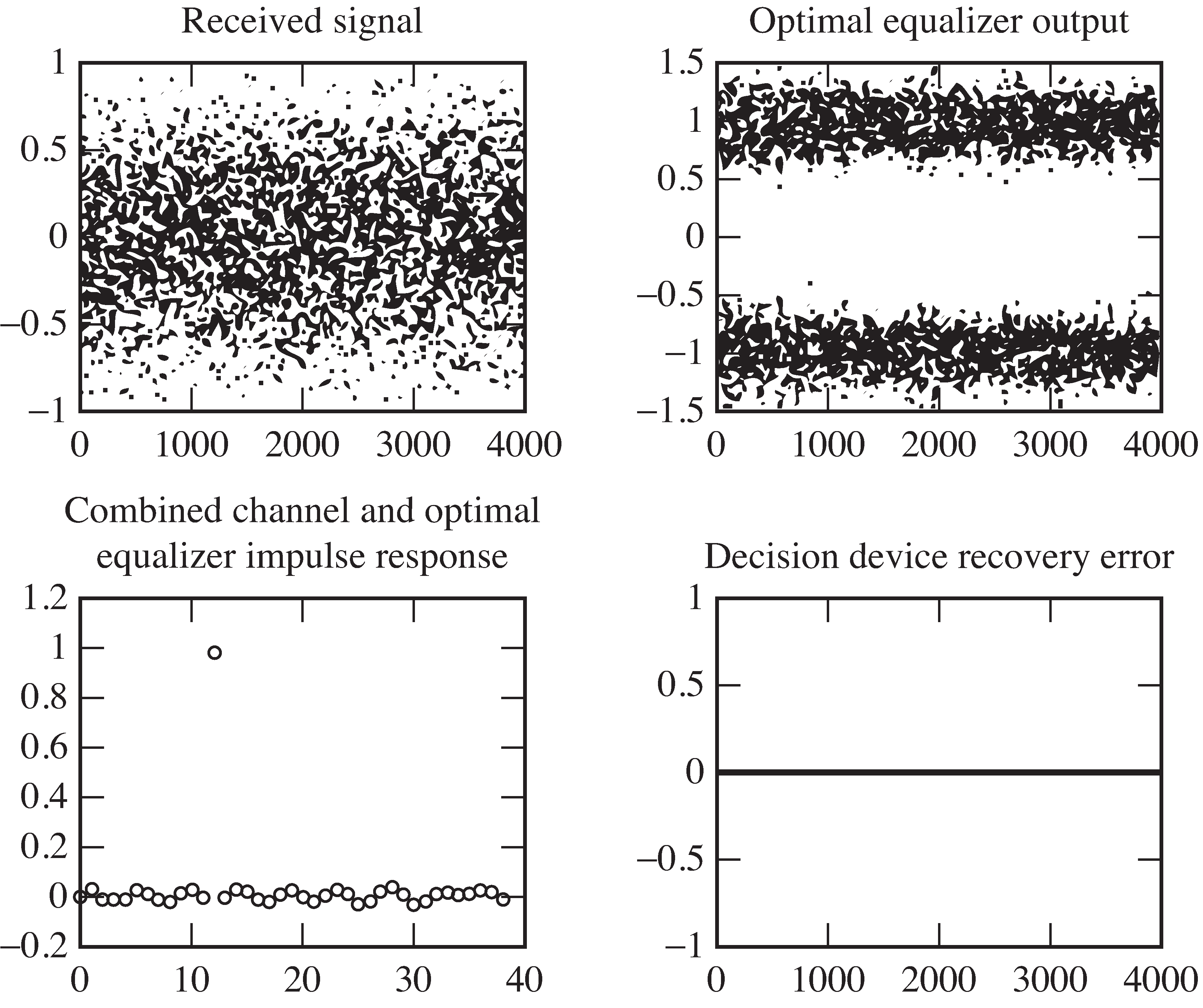
— is the frequency response of the equalizer, and the solid lineis the frequency response of the combined channel–equalizer pair.Trained least-squares equalizer for Channel 1: Time responses.
As in
[link] , the equalizer is able to effectively
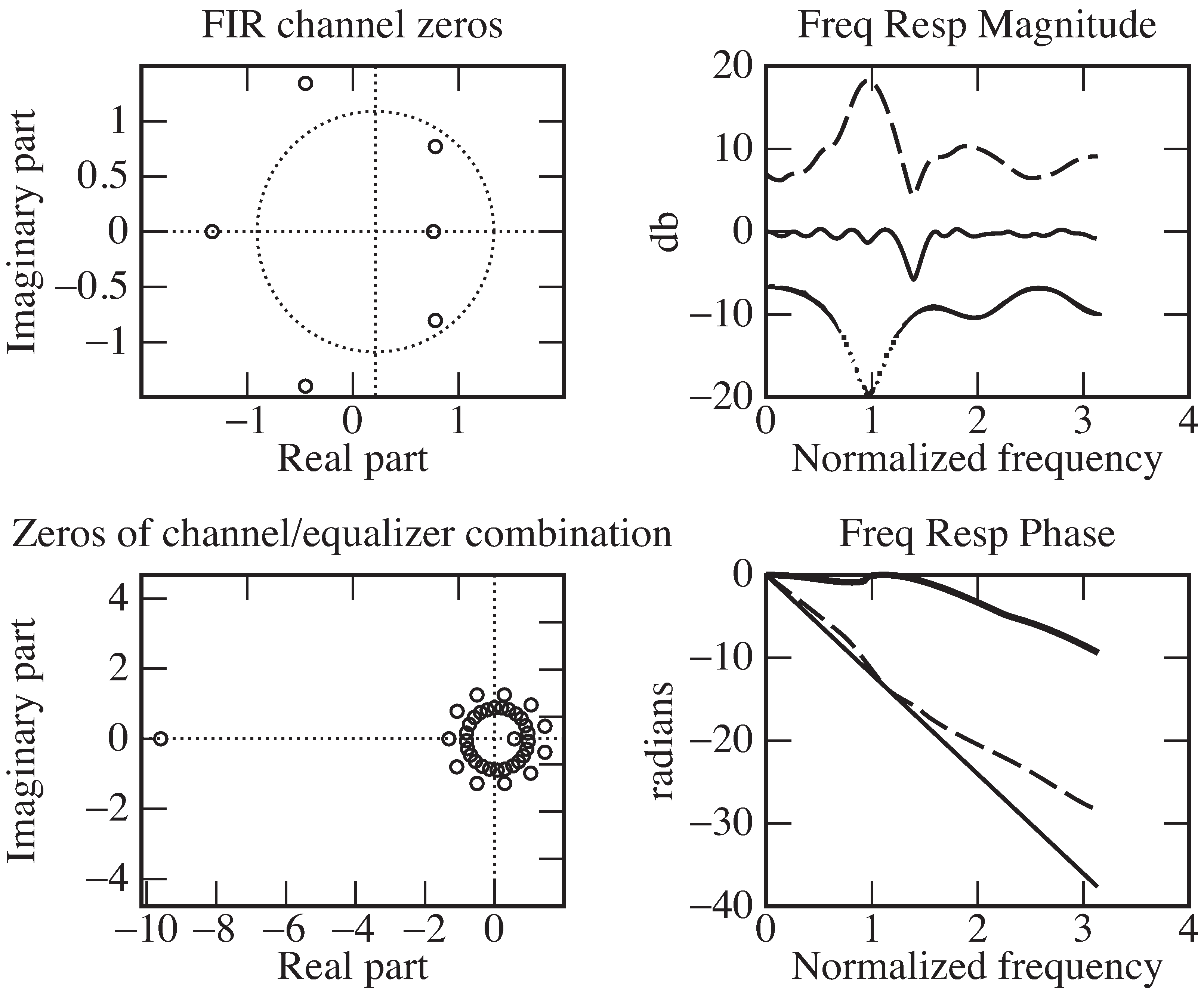
undo the effects of the channel.Trained least-squares equalizer for Channel 1: Singularities and
frequency responses. The large circles show the locations of thezeros of the channel in the upper left plot and the locations of the
zeros of the combined channel–equalizer pair in the lower left.The *** represents the frequency response of the channel,
— is the frequency response of the equalizer, and the solid lineis the frequency response of the combined channel–equalizer pair.Trained least-squares equalizer for Channel 2: Time responses.
Even for this farily severe channel, the equalizer is able to effectivelyundo the effects of the channel as in Figures
[link] and
[link] .Trained least-squares equalizer for Channel 2: Singularities
and frequency responses. The large circles show the locations of thezeros of the channel in the upper left plot and the locations of the
zeros of the combined channel–equalizer pair in the lower left.The *** represents the frequency response of the channel,
— is the frequency response of the equalizer, and the solid lineis the frequency response of the combined channel–equalizer pair.
Channel 1
condition number: 14.795
minimum value of performance function: 0.0307
optimum delay: 12
percentage of errors: 0
Channel 2
condition number: 164.1081
minimum value of performance function: 0.0300
optimum delay: 10
percentage of errors: 0
Questions & Answers
differentiate between demand and supply
giving examples
In economics, a perfect market refers to a theoretical construct where all participants have perfect information, goods are homogenous, there are no barriers to entry or exit, and prices are determined solely by supply and demand. It's an idealized model used for analysis,
When MP₁ becomes negative, TP start to decline.
Extuples Suppose that the short-run production function of certain cut-flower firm is given by: Q=4KL-0.6K2 - 0.112 •
Where is quantity of cut flower produced, I is labour input and K is fixed capital input (K-5). Determine the average product of lab
Kelo
Extuples Suppose that the short-run production function of certain cut-flower firm is given by: Q=4KL-0.6K2 - 0.112 •
Where is quantity of cut flower produced, I is labour input and K is fixed capital input (K-5). Determine the average product of labour (APL) and marginal product of labour (MPL)
Quantity demanded refers to the specific amount of a good or service that consumers are willing and able to purchase at a give price and within a specific time period. Demand, on the other hand, is a broader concept that encompasses the entire relationship between price and quantity demanded
Ezea
ok
Shukri
how do you save a country economic situation when it's falling apart
Economic growth as an increase in the production and consumption of goods and services within an economy.but
Economic development as a broader concept that encompasses not only economic growth but also social & human well being.
Shukri
production function means
Jabir
What do you think is more important to focus on when considering inequality ?
sir...I just want to ask one question... Define the term contract curve? if you are free please help me to find this answer 🙏
Asui
it is a curve that we get after connecting the pareto optimal combinations of two consumers after their mutually beneficial trade offs
Awais
thank you so much 👍 sir
Asui
In economics, the contract curve refers to the set of points in an Edgeworth box diagram where both parties involved in a trade cannot be made better off without making one of them worse off. It represents the Pareto efficient allocations of goods between two individuals or entities, where neither p
Cornelius
In economics, the contract curve refers to the set of points in an Edgeworth box diagram where both parties involved in a trade cannot be made better off without making one of them worse off. It represents the Pareto efficient allocations of goods between two individuals or entities,
Cornelius
Suppose a consumer consuming two commodities X and Y has
The following utility function u=X0.4 Y0.6. If the price of the X and Y are 2 and 3 respectively and income Constraint is birr 50.
A,Calculate quantities of x and y which maximize utility.
B,Calculate value of Lagrange multiplier.
C,Calculate quantities of X and Y consumed with a given price.
D,alculate optimum level of output .
the market for lemon has 10 potential consumers, each having an individual demand curve p=101-10Qi, where p is price in dollar's per cup and Qi is the number of cups demanded per week by the i th consumer.Find the market demand curve using algebra. Draw an individual demand curve and the market dema
suppose the production function is given by ( L, K)=L¼K¾.assuming capital is fixed find APL and MPL. consider the following short run production function:Q=6L²-0.4L³ a) find the value of L that maximizes output b)find the value of L that maximizes marginal product