0.10 Numerical simulation  (Page 3/8)

If the boundary condition is that of zero vorticity as on a surface of symmetry, it is necessary to only set to zero the coefficient that multiplies the boundary value of vorticity, i.e.,

$\begin{array}{c}i=2\hfill \\ b(i,j,2,2)=0,\mathrm{when}w(1,j)=0\hfill \end{array}$

The linear system of equations and unknowns can be written in matrix form by ordering the equations with the i index changing the fastest, i.e., $i=2,3, ,JMAX-1$ . The linear system of equations can now be expressed in matrix notation as follows.

The non-zero coefficients of coefficient matrix A for $JMAX=5$ is illustrated below. Since the first and last grid points of each row and column of grid points are boundary conditions, the number of grid with pairs of unknowns is only 3x3. Only one grid point is isolated from boundaries. The $i$ , $j$ location of the coefficients become clearer if a box is drawn to enclose each $2x2$ coefficient.

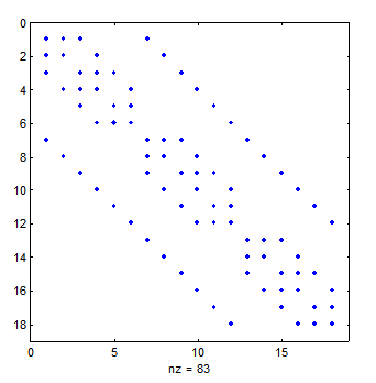
Most of the elements of the coefficient matrix are zero. In fact, the coefficient matrix is a block pentadiagonal sparse matrix and only the nonzero coefficients need to be stored and processed for solving the linear system of equations. The non-zero coefficients of the coefficient matrix are stored with the row-indexed sparse storage mode and the linear system of equations is solved by preconditioned biconjugate gradient method (Numerical Recipes, 1992).

The row-indexed sparse matrix mode requires storing the nonzero coefficients in the array, $sa\left(k\right)$ , and the column number of the coefficient in the coefficient matrix in the array, $ija\left(k\right)$ , where $k=1,2,$ . The indices that are needed to identify the coefficients are the $i,j$ grid location $(i,j=2,3, ,JMAX-1)$ , the $m$ equation and dependent variable identifier ( $m=1$ for stream function; $=2$ for vorticity), and the $IA$ row index of the coefficient matrix $(IA=1,2,3,4, ,2(JMAX-2\left)2\right)$ . The coefficient matrix has two equations for each grid point, the first for the stream function and the second for vorticity. The total number of equations is $NN=2(JMAX-2)2$ .

The diagonal elements of the coefficient array are first stored in the $sa\left(k\right)$ array. The first element of $ija\left(k\right)$ , $ija\left(1\right)=NN+2$ and can be used to determine the size of the coefficient matrix. The algorithm then cycles over the pairs of rows in the coefficient matrix while keeping track of the $i$ , $j$ locations of the grid point and cycling over equation $m=1\text{and}2$ . The off-diagonal coefficients are stored in $sa\left(k\right)$ and the column number in the coefficient matrix stored in $ija\left(k\right)$ . As each row is completed, the $k$ index for the next row is stored in the first $NN$ elements of $ija$ .

A test problem for this code is a square box that has one side sliding as to impart a unit tangential component of velocity along this side. All other walls are stationary. The stream function, vorticity, and velocity contours for this problem with a 20x20 grid is illustrated below.