0.10 Lecture 11:sinusoidal steady-state (sss) or frequency response  (Page 3/5)

And

$\begin{array}{}\text{arg}(H(\mathrm{j\omega }))=\text{arg}(K)+\text{arg}(j{\text{ωτ}}_{\mathrm{z1}}+1)+\text{arg}(j{\text{ωτ}}_{\mathrm{z2}}+1)+\text{.}\text{.}\text{.}+\text{arg}(j{\text{ωτ}}_{\text{zM}}+1)\\ \begin{array}{cc}\begin{array}{cc}\begin{array}{cc}\begin{array}{cc}& \end{array}& \end{array}& \end{array}& \end{array}-\text{arg}(j{\text{ωτ}}_{\mathrm{p1}}+1)-\text{arg}(j{\text{ωτ}}_{\mathrm{p2}}+1)-\text{.}\text{.}\text{.}-\text{arg}(j{\text{ωτ}}_{\text{pN}}+1)\end{array}$

4/ Logarithmic magnitude

Taking twenty times the logarithm of the magnitude yields

$\begin{array}{}\text{20}{\text{log}}_{\text{10}}\mid H(\mathrm{j\omega })\mid =\text{20}{\text{log}}_{\text{10}}\mid K\mid +\text{20}{\text{log}}_{\text{10}}\mid j{\text{ωτ}}_{\mathrm{z1}}+1\mid +\text{20}{\text{log}}_{\text{10}}\mid j{\text{ωτ}}_{\mathrm{z2}}+1\mid +\text{.}\text{.}\text{.}+\text{20}{\text{log}}_{\text{10}}\mid j{\text{ωτ}}_{\text{zM}}+1\mid \\ \begin{array}{cc}\begin{array}{cc}\begin{array}{cc}\begin{array}{cc}& \end{array}& \end{array}& \end{array}& \end{array}-\text{20}{\text{log}}_{\text{10}}\mid j{\text{ωτ}}_{\mathrm{p1}}+1\mid -\text{20}{\text{log}}_{\text{10}}\mid j{\text{ωτ}}_{\mathrm{p2}}+1\mid -\text{.}\text{.}\text{.}-\text{20}{\text{log}}_{\text{10}}\mid j{\text{ωτ}}_{\text{pN}}+1\mid \end{array}$

Note than both the logarithmic magnitude and the angle are expressed as sums of terms of the form

$\pm {\text{20 log}}_{\text{10}}\mid j\text{ωτ}+1\mid \begin{array}{cc}& \end{array}\text{and}\begin{array}{cc}& \end{array}\pm \text{arg}(j\text{ωτ}+1)$

Therefore, to plot the frequency response we need to add terms of the above form.

5/ Decibels

It is common to plot frequency responses as Bode diagrams whose magnitude is expressed in decibels. The decibel, denoted by dB, is defined as ${\text{20 log}}_{\text{10}}\mid {\rm H}\mid$ . The following table gives decibel equivalents for a few quantities.

How many decibels correspond to |H| = 50? Express |H| =100/2. Then

${\text{20 log}}_{\text{10}}(\text{100/2})={\text{20 log}}_{\text{10}}{\text{100 - 20log}}_{\text{10}}\text{2}\approx \text{40}\text{- 6}\text{=}\text{34}\text{dB}$

6/ Asymptotes

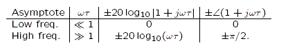
To plot the frequency response of a system with real poles and zeros, we need to plot terms of the form

$\pm {\text{20 log}}_{\text{10}}\mid 1+j\text{ωτ}\mid \begin{array}{cc}& \end{array}\text{and}\begin{array}{cc}& \end{array}\pm \text{arg}(1+j\text{ωτ})$

The low and high frequency asymptotes are

7/ Corner frequency

At $\omega \text{=}{\omega }_c\text{= 1}/\tau$ , called the corner or cut-off frequency,

• the low- and high-frequency asymptotes intersect,

• the magnitude is

$\pm {\text{20 log}}_{\text{10}}\mid \text{1+j}\text{ωτ}\mid \text{=}\pm {\text{20 log}}_{\text{10}}\mid \text{1+j1}\mid \text{=}\pm {\text{20 log}}_{\text{10}}{2}^{\text{1/2}}\pm \text{3 dB}$

• the angle is

$\pm \text{arg}(\text{1+}j\text{ωτ})\text{=}\pm \text{arg}(\text{1+}j)\text{=}\pm \pi /4$

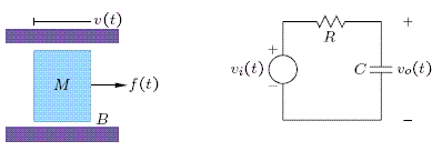
Example — first-order lowpass system

First-order low pass systems arise in a large variety of physical contexts. For example,

For the parameters M = B = R = C = 1, the frequency responses for the two systems are

$H(\mathrm{j\omega })=\frac{V(\mathrm{j\omega })}{F(\mathrm{j\omega })}=\frac{1}{\mathrm{j\omega }+1}\begin{array}{cc}& \end{array}\text{and}\begin{array}{cc}& \end{array}H(\mathrm{j\omega })=\frac{V_0(\mathrm{j\omega })}{V_i(\mathrm{j\omega })}=\frac{1}{\mathrm{j\omega }+1}$

Magnitude

For

$H(\mathrm{j\omega })=\frac{1}{\mathrm{j\omega }+1}$

the low-frequency asymptote has a slope of 0 and an intercept of 0 dB and the high-frequency asymptote has a slope of -20 dB/decade and an intercept of 0 dB at the corner frequency.

The corner frequency is 1 rad/sec and the bandwidth is 1 rad/sec. The two asymptotes intersect at ω = 1 where ${\text{20 log}}_{\text{10}}\mid {\rm H}(\text{jω})\mid \text{=}\text{-3}\text{dB}$

$H(\mathrm{j\omega })=\frac{1}{\mathrm{j\omega }+1}$

the low- and high-frequency asymptotes of the angle of the frequency response are 0 and $-{\text{90}}^0$ (−π/2 radians), respectively. The angle is $-{\text{45}}^0$ at the corner frequency (1 rad/sec).

A line drawn from the low frequency asymptote a decade below the corner frequency to the high frequency asymptote a decade above the corner frequency approximates the angle of the frequency response.

Physical interpretation

With M = B = 1, the frequency response is

$H(\mathrm{j\omega })=\frac{V(\mathrm{j\omega })}{F(\mathrm{j\omega })}=\frac{1}{\mathrm{j\omega }+1}$

At low frequencies, |H(jω)| → 1 and arg H(jω) → 0. The inertia of the mass is negligible, and the damping force dominates so that the external force is proportional to velocity.

At high frequencies, |H(jω)| → 1/ω and arg H(jω) → $-{\text{90}}^0$ . The inertia of the mass dominates so that the acceleration is proportional to external force and the velocity decreases as frequency increases.

With R = C = 1, the frequency response is

$$ $H(\mathrm{j\omega })=\frac{V_o(\mathrm{j\omega })}{V_i(\mathrm{j\omega })}=\frac{1}{\mathrm{j\omega }+1}$

At low frequencies, |H(jω)| → 1 and arg H(jω) → 0. The impedance of the capacitance is large so that all the input voltage appears at the output.

At high frequencies, |H(jω)| → 1/ω and arg H(jω) → $-{\text{90}}^0$ . The impedance of the capacitance is small so that the current is determined by the resistance and the output voltage is determined by the impedance of the capacitance which decreases as frequency increases.