0.10 Lecture 11:sinusoidal steady-state (sss) or frequency response  (Page 2/5)

2/ H(s) along the imaginary axis

H(s) evaluated for s = jω or H(jω) is called the frequency response.

3/ Radian frequency and frequency

• ω is the radian frequency in units of radians/second.

• ω can be expressed as ω = 2πf.

• f is the frequency in units of cycles per second which is called hertz (Hz).

• The frequency response H(j2πf) is often plotted versus f.

4/ Measurement of H(jω)

To measure H(jω) of a test system we can use the system shown below.

However, when the sinusoid is turned on the response contains both a transient and a steady-state component.

For example, suppose

$H(s)=\frac{\mathrm{5s}}{(s+1{)}^2+{\text{10}}^2}$

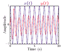
The response of this system, y(t), to the input x(t) = cos(2πt) u(t) is shown below.

Note the transient at the onset which damps out after a few cycles of the sinusoid so that the response approaches the particular solution, i.e., this is the steady-state response.

Therefore, to measure H(jω) we turn on the oscillator and wait till steady state is established and measure the input and output sinusoid. At each frequency, the ratio of the magnitude of the output to the magnitude of the input sinusoid defines the magnitude of the frequency response. The angle of the output minus that of the input defines the angle of the frequency response.

More elaborate systems are available for measuring the frequency response rapidly and automatically.

5/ Relation of time waveforms, vector diagrams, and frequency response

Consider and LTI system with system function

$H(s)=\frac{1}{s+1}$

which has the frequency response

$H(\mathrm{j\omega })=\frac{1}{\mathrm{j\omega }+1}$

The input is

$x(t)\text{cos}(\mathrm{\omega t})$

and the response is

$\begin{array}{}y(t)=\mid H(\mathrm{j\omega })\mid \text{cos}(\mathrm{\omega t}+\text{arg}H(\mathrm{j\omega }))\\ y(t)=\frac{1}{({\omega }^2+1{)}^{1/2}}\text{cos}(\mathrm{\omega t}-{\text{tan}}^{-1}\omega )\end{array}$

Demo of relation of pole-zero diagram, time waveforms, vector diagrams, and frequency response.

6/ Different ways of plotting the frequency response

The frequency response H(jω) = 1/(jω +1), is plotted in linear coordinates (left) and in doubly logarithmic coordinates called a Bode diagram (right).

IV. BODE DIAGRAMS

1/ Definition and rationale

Frequency responses are commonly plotted as Bode diagrams which are plots of

$\text{20}{\text{log}}_{\text{10}}\mid H(\mathrm{j\omega })\mid$ plotted versus ${\text{log}}_{\text{10}}\omega$

$\text{arg}H(\mathrm{j\omega })$ plotted versus ${\text{log}}_{\text{10}}\omega$ .

The reasons are:

• Logarithmic coordinates are useful when the range of |H(jω)| and/or ω is large.

• Asymptotes to the frequency response are easily plotted.

• When the poles and zeros are on the real axis, the asymptotes are excellent approximations to the frequency response.

2/ Pole-zero and time-constant form

Consider an LTI system whose system function has poles and zeros on the negative, real axis. It can be displayed in pole-zero form as follows

$H(s)=C\frac{(s+z_1)(s+z_2)\text{.}\text{.}\text{.}(s+z_M)}{(s+p_1)(s+p_2)\text{.}\text{.}\text{.}(s+p_N)}$

This system function can be evaluated along the jω axis to yield

$H(s)=C\frac{(\mathrm{j\omega }+z_1)(\mathrm{j\omega }+z_2)\text{.}\text{.}\text{.}(\mathrm{j\omega }+z_M)}{(\mathrm{j\omega }+p_1)(\mathrm{j\omega }+p_2)\text{.}\text{.}\text{.}(\mathrm{j\omega }+p_N)}$

By dividing the numerator by each zero and the denominator by each pole, the frequency response can be put in time-constant form as follows

$H(\mathrm{j\omega })=K\frac{(j{\text{ωτ}}_{\mathrm{z1}}+1)(j{\text{ωτ}}_{\mathrm{z2}}+1)\text{.}\text{.}\text{.}(j{\text{ωτ}}_{\text{zM}}+1)}{(j{\text{ωτ}}_{\mathrm{p1}}+1)(j{\text{ωτ}}_{\mathrm{p2}}+1)\text{.}\text{.}\text{.}(j{\text{ωτ}}_{\text{pN}}+1)}$

3/ Magnitude and angle

The magnitude and angle can be expressed as

$\mid H(\mathrm{j\omega })\mid =\mid K\mid \frac{\mid j{\text{ωτ}}_{\mathrm{z1}}+1\mid \mid j{\text{ωτ}}_{\mathrm{z2}}+1\mid \text{.}\text{.}\text{.}\mid j{\text{ωτ}}_{\text{zM}}+1\mid }{\mid j{\text{ωτ}}_{\mathrm{p1}}+1\mid \mid j{\text{ωτ}}_{\mathrm{p2}}+1\mid \text{.}\text{.}\text{.}\mid j{\text{ωτ}}_{\text{pN}}+1\mid }$