

| << Chapter < Page | Chapter >> Page > |
As mentioned in [link] , one can address problem [link] in two ways depending on how one views the role of the transition band in a CLS problem. The original problem posed by Adams in [link] can be written as follows,
where . From a traditional standpoint this formulation feels familiar. It assigns fixed frequencies to the transition band edges as a number of filter design techniques do. As it turns out, however, one might not want to do this in CLS design.
An alternate formulation to [link] could implicitly introduce a transition frequency (where ); the user only specifies . Consider
The algorithm at each iteration generates an induced transition band in order to satisfy the constraints in [link] . Therefore vary at each iteration.
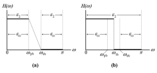
It is critical to point out the differences between [link] and [link] . [link] .a explains Adams' CLS formulation, where the desired filter response is only specified at the fixed pass and stop bands. At any iteration, Adams' method attempts to minimize the least squares error ( ) at both bands while trying to satisfy the constraint . Note that one could think of the constraint requirements in terms of the Chebishev error by writing [link] as follows,
In contrast, [link] .b illustrates our proposed problem [link] . The idea is to minimize the least squared error across all frequencies while ensuring that constraints are met in an intelligent manner. At this point one can think of the interval as an induced transition band, useful for the purposes of constraining the filter. [link] presents the actual algorithms that solve [link] , including the process of finding .
It is important to note an interesting behavior of transition bands and extrema points in
and
filters.
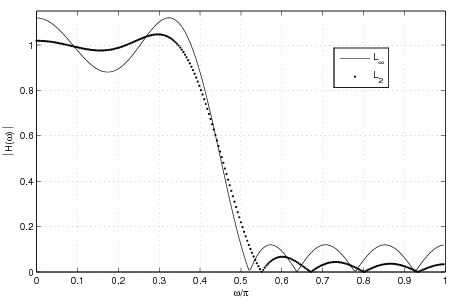
[link] shows
and
length-15 linear phase filters (designed using Matlab's
firls and
firpm functions); the transition band was specified at
. The dotted
filter illustrates an important behavior of least squares filters: typically the maximum error of an
filter is located at the transition band. The solid
filter shows why minimax filters are important: despite their larger error across most of the bands, the filter shows the same maximum error at all extrema points, including the transition band edge frequencies. In a CLS problem then, typically an algorithm will attempt to reduce iteratively the maximum error (usually located around the transition band) of a series of least squares filters.
Another important fact results from the relationship between the transition band width and the resulting error amplitude in filters. [link] shows two designs; the transition bands were set at for the solid line design, and at for the dotted line one. One can see that by widening the transition band a decrease in error ripple amplitude is induced.
Notification Switch
Would you like to follow the 'Iterative design of l_p digital filters' conversation and receive update notifications?

|
|

|
|

|
|

|
|

|
|

|
|

|
|

|
|

|
|

|