0.1 Lecture 2: introduction to systems  (Page 5/8)

Y=H(s)X

where

$H(s)=\frac{\sum _{m=0}^M{b}_m{s}^m}{\sum _{n=0}^N{a}_n{s}^n}$

b/ System function definition

$H(s)=\frac{\sum _{m=0}^M{b}_m{s}^m}{\sum _{n=0}^N{a}_n{s}^n}$

• is called the system function

• is a rational function in s

• is a skeleton of the differential equation

• characterizes the relation between x(t) and y(t)

Example — reconstruction of differential equation from H(s)

Suppose

$H(s)=\frac{Y}{X}=\frac{s}{s+1}$

what is the differential equation that relates y(t) to x(t)? Cross-multiply the equation and multiply both sides by $e^{\text{st}}$ to obtain

$(s+1){\text{Ye}}^{\text{st}}={\text{sXe}}^{\text{st}}$

which yields

${\text{sYe}}^{\text{st}}+{\text{Ye}}^{\text{st}}={\text{sXe}}^{\text{st}}$

from which we can obtain the differential equation

$\frac{\text{dy}(t)}{\text{dt}}+y(t)=\frac{\text{dx}(t)}{\text{dt}}$

2/ Poles and zeros

H(s) can be expressed in factored form as follows

$H(s)=K\frac{\prod _{m=1}^M(s-z_m)}{\prod _{n-1}^N(s-p_n)}$

where $K=\frac{b_M}{a_M}$

• $\{z_1,z_2,\text{.}\text{.}\text{.},z_M\}$ are the roots of the numerator polynomial and are called zeros of H(s) because these are the values of s for which H(s) = 0.

• $\{p_1,p_2,\text{.}\text{.}\text{.},p_M\}$ are the roots of the denominator polynomial and are called poles of H(s) because these are the values of s for which $H(s)=\infty$ .

a/ Poles are the natural frequencies

Note that poles of H(s) are the natural frequencies of the system. Recall that natural frequencies are given by the roots of the characteristic polynomial

$(\sum _{n=0}^N{a}_n{\lambda }^n)=0$

and the poles are the roots of denominator polynomial of H(s)

$(\sum _{n=0}^N{a}_n{s}^n)=0$

Both originate from the left-hand side of the differential equation

$\sum _{n=0}^N{a}_n\frac{d^{n}y(t)}{{\text{dt}}^n}$

b/ Pole-zero diagram

H(s) characterizes the differential equation and H(s) is characterized by N + M + 1 numbers: N poles, M zeros, and the constant K. Except for the multiplication factor K, H(s) is characterized by a pole-zero diagram which is a plot of the locations of poles and zeros in the complex-s plane. The ordinate is $\text{jI}\{s\}=\mathrm{j\varpi }$ and the abscissa is $R\{s\}=\sigma$ where

$s=\sigma +\mathrm{j\varpi }$

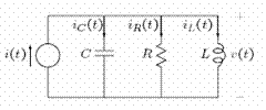
Example — system function of a network

The differential equation relating v(t) to i(t) is

$\frac{\text{di}(t)}{\text{dt}}=C(\frac{d^{2}v(t)}{{\text{dt}}^2}+\frac{1}{\text{RC}}\frac{\text{dv}(t)}{\text{dt}}+\frac{v(t)}{\text{LC}})$

The particular solution is obtained from

$\text{sI}=C(s^2+\frac{1}{\text{RC}}s+\frac{1}{\text{LC}})V$

With v(t) as the output and i(t) as the input, the system function of the RLC network is

$H(s)=\frac{V}{I}=\frac{1}{C}(\frac{s}{s^2+\frac{1}{\text{RC}}s+\frac{1}{\text{LC}}})$

Two-minute miniquiz problem

Problem 3-1

Given the system function

$H(s)=\frac{s+2}{(s+3)(s+4)}$

• Determine the natural frequencies of the system.
• Determine a differential equation that relates x(t) and y(t).

Solution

• The natural frequencies of the system are the poles of the system function and are −3 and −4.
• The differential equation can be obtained by cross multiplying and multiplying by $e^{\text{st}}$ to obtain

$(s+3)(s+4){\text{Ye}}^{\text{st}}=(s+2){\text{Xe}}^{\text{st}}$

$(s^2+\mathrm{7s}+\text{12}){\text{Ye}}^{\text{st}}=(s+2){\text{Xe}}^{\text{st}}$

so that

$\frac{d^{2}y(t)}{{\text{dt}}^2}+7\frac{\text{dy}(t)}{\text{dt}}+\text{12}y(t)=\frac{\text{dx}(t)}{\text{dt}}+\mathrm{2x}(t)$

VIII. TOTAL SOLUTION

The general solution is

$y(t)=\sum _{n=1}^N{A}_n{e}^{{\lambda }_{n}t}+\text{XH}(s)e^{\text{st}}\text{for}t>0$

and

y(t)=0 for t<0

Hence, provided there are no singularity functions (e.g., impulses) at t = 0, the general solution can be written compactly as follows

$y(t)=(\sum _{n=1}^N{A}_n{e}^{{\lambda }_{n}t}+\text{XH}(s)e^{\text{st}})u(t)$

As we shall see later, no singularity functions occur in the response provided the order of the numerator polynomial of H(s) does not exceed that of the denominator.

1/ Initial conditions

To completely determine the total solution we need to determine the N coefficients

$\{A_1,A_2,\text{.}\text{.}\text{.},A_N\}$