

| << Chapter < Page | Chapter >> Page > |
Start Matlab on your workstation and type the following sequence of commands.
n = 0:2:60;
y = sin(n/6);subplot(3,1,1)
stem(n,y)
This plot shows the discrete-time signal formed by computing the values of the function at points which are uniformly spaced at intervals of size 2.Notice that while is a continuous-time function, the sampled version of the signal, , is a discrete-time function.
A digital computer cannot store all points of a continuous-time
signal since this would require an infinite amount of memory.It is, however, possible to plot a signal which
looks like a continuous-time signal, by computing
the value of the signal at closely spaced points in time,and then connecting the plotted points with lines.
The Matlab
plot function may be used to generate
such plots.
Use the following sequence of commands to generate two continuous-time plots of the signal .
n1 = 0:2:60;
z = sin(n1/6);subplot(3,1,2)
plot(n1,z)n2 = 0:10:60;
w = sin(n2/6);subplot(3,1,3)
plot(n2,w)
As you can see, it is important to have many pointsto make the signal appear smooth. But how many points are enough for numerical calculations?In the following sections we will examine the effect of the sampling interval on the accuracyof computations.
title command, and include your names.
Comment on the accuracy of each of the continuous timeplots.For help on the following topics, click the corresponding link: MatLab Scripts , MatLab Functions , and the Subplot Command .
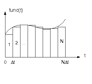
To see the effects of using a different number of points
to represent a continuous-time signal,write a Matlab function
for numerically computing the integralof the function
over the interval
.
The syntax of the function should be
I=integ1(N) where
is the result and
is the number of rectanglesused to approximate the integral.
This function should use the
sum command
and it should
not contain any
for loops!
Next write an m-file script that evaluates for , stores the result in a vector and plots the resulting vector as a function of . This m-file script may contain for loops.
Repeat this procedure for a second function
J=integ2(N) which numerically computes the integral of
on the interval
.
Notification Switch
Would you like to follow the 'Purdue digital signal processing labs (ece 438)' conversation and receive update notifications?

|
|

|
|

|
|

|
|

|
|

|
|

|
|

|
|
|
|
|

|