0.1 Background  (Page 2/2)

The convolution in question is:

The Gaussian function is:

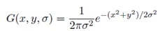
Note that in G(x, y, σ), x and y actually represent the distance of the current pixel from the origin in the x and y directions, respectively. For I(x, y), x and y are simply the coordinates of the current pixel. As σ increases, the amount of blur and thus the type of scale that is preserved increases. Some example Matlab code is as follows:

Source = im2double(rgb2gray(imresize(imread('MainImage.jpg'),[480,640])));

Variance = 100;

for x=1:480

for y=1:640

R(x,y) = (1/sqrt(2*pi*Variance))*exp((-(abs(x-240)^2+abs(y-320)^2))/(2*Variance));

end

end

Blurred = conv2(Source,R)/(2*sqrt(Variance));

imshow(Blurred)

The convolution of the image with the Gaussian will not be the same size as the original image, so cropping is necessary to get something like the bottom image. Additionally, convolving by the Gaussian function in 2-D is separable, which means that using a convolution matrix to get the 2-D convolution gives the same result as applying a 1-D convolution in both directions. This is useful because it makes computation much, much faster, but it is also a bit more involved. Matlab takes care of all these issues through the fspecial and imfilter functions. For example, the previous code can be replaced with the following:

Source = im2double(rgb2gray(imresize(imread('MainImage.jpg'),[480,640])));

Variance = 100;

h = fspecial('gaussian',[480,640],sqrt(Variance));

imfilter(Source,h); %convolves source with h and performs necessary cropping

imshow(ans);

Later Steps

SIFT operates on grayscale images because for each pixel only one byte of information is required (intensity) so the convolutions are a lot faster. It is also worth mentioning that the size of the Gaussian filter used doesn't need to be the size of the entire image, but larger filters result in stronger blur. In SIFT, the original image is downsampled by increasing factors of 2, and each of these images is then blurred to different levels. The number of downsampled images is called the number of "octaves", and can be chosen by the programmer. Normally 4 octaves are used with 5 levels of blur each for a total of 20 images.

The next step involves taking the difference of these blurred images. In each octave, each image has its neighbor with a higher level of blur subtracted from itself except the last one since there is nothing after it. The effect of this step is leaving an image where edges, corners, and other features have higher contrast than places that are less well defined.

Example:

h1 = fspecial('gaussian',[8,8],1.5);

h2 = fspecial('gaussian',[8,8],10);

LowBlur = imfilter(Source,h1);

HighBlur = imfilter(Source,h2);

imshow(HighBlur-LowBlur);

From these Difference of Gaussian (DoG) images, minima and maxima are located; these are the initial sets of keypoints. Next, a contrast check is done that throws away keypoints that are not above some threshold contrast with respect to their neighboring pixels; this helps increase the accuracy of the algorithm. Lastly, for each keypoint, descriptors including scale and orientation are calculated by using neighboring pixels.

An important difference between SIFT and SURF is that SURF does not downsample images by factors of 2 and instead just keeps a "stack" of images at the same resolution, but with different levels of blur. Then, instead of finding the difference of Gaussians, SURF approximates second-order derivatives by using boxcar filters; this results in a much higher calculation speed, but with sometimes lower rates of detection accuracy.

Fortunately, there are many implementations of SURF available in various programming languages. In initial testing during this project, OpenCV's C++ implementation of the algorithm was used, and it was almost fast enough to track in real time using a 640x480 resolution webcam input. Since a lot of the sound code we already had was done in Matlab, however, we instead opted for Dirk-Jan Kroon's Matlab adaptation of OpenSURF, originally a very fast C++ implementation by Chris Evans.

Example Results

The 3-d sound effect

Definition

The 3-D sound effect allows the listener to locate the exact position of an object in space. The position is described in terms of an azimuth and elevation. The following figure illustrates the concepts of azimuth and elevation, as well as the spatial coordinate system we used in our project.

One of the most common ways to synthesize 3-D sound is to use the head-related transfer function, which includes information about the interaural time difference (ITD), interaural intensity difference, and spectral coloration of a sound made by the torso, head, outer ears, or pinna. The interaural time difference is defined to be the difference in time between when the wavefront arrives at the left ear and when the wavefront arrives at the right ear (Figure 7). The source of sound is perceived to be closer to the ear at which the first wavefront arrives. As such, a larger ITD corresponds to a larger lateral displacement.

Using ITD, we can decide the azimuth of the sound source. Unfortunately, when the frequency is above 1500 Hz, the wavelength of the sound is approximately the diameter of the head. Therefore, different azimuths might have the same ITD, and aliasing will occur (Figure 8).

In order to uniquely determine the lateral position of the sound source, the interaural intensity difference (IID) is introduced to the HRTF. The interaural intensity difference is defined as the amplitude difference between the wavefront that arrived at the left ear and the wavefront that arrived at the right ear (Figure 9).

Utilizing both ITD and IID, we can find the azimuth of the sound source, but not its position in space. In fact, there are infinitely many points in space which have the same ITD and IID. Those points form a so-called “cone of confusion” (Figure 10).

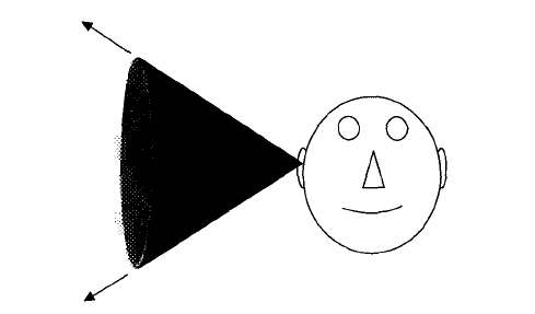
In order to distinguish sounds originating from points on a cone of confusion, the HRTF we used in our project includes the spectral cues produced by the structure of the ears. With the ITD, IID, and these spectral cues, our system can exactly locate the position of sound source in space.