Figure 1
Published: April 18, 2006
by Richard G. Baldwin
Java Programming Notes # 2360
DSP and adaptive filtering
With the decrease in cost and the increase in speed of digital devices, Digital Signal Processing (DSP) is showing up in everything from cell phones to hearing aids to rock concerts. Many applications of DSP are static. That is, the characteristics of the digital processor don't change with time or circumstances. However, a particularly interesting branch of DSP is adaptive filtering. This is a scenario where the characteristics of the digital processor change with time, circumstances, or both.
Sixth in a series
This is the sixth lesson in a series designed to teach you about adaptive filtering in Java. The first lesson, titled Adaptive Filtering in Java, Getting Started, introduced you to the topic by showing you how to write a Java program to adaptively design a time-delay convolution filter with a flat amplitude response and a linear phase response using an LMS adaptive algorithm.
A general-purpose adaptive engine
The third lesson in the series, titled A General-Purpose LMS Adaptive Engine in Java, presented and explained a general-purpose LMS adaptive engine written in Java. That engine can be used to solve a wide variety of adaptive problems.
Adaptive identification and inverse filtering
The previous lesson titled Adaptive Identification and Inverse Filtering using Java showed you how to accomplish the first two items in the following list of common applications of adaptive filtering:
Adaptive noise cancellation
This lesson presents and explains a program named Adapt08, which demonstrates the use of adaptive filtering for the third item in the above list, Noise Cancellation. A future lesson will deal with the last item in the above list, Prediction.
Viewing tip
You may find it useful to open another copy of this lesson in a separate browser window. That will make it easier for you to scroll back and forth among the different listings and figures while you are reading about them.
Supplementary material
I recommend that you also study the other lessons in my extensive collection of online Java tutorials. You will find those lessons published at Gamelan.com. However, as of the date of this writing, Gamelan doesn't maintain a consolidated index of my Java tutorial lessons, and sometimes they are difficult to locate there. You will find a consolidated index at www.DickBaldwin.com.
In preparation for understanding the material in this lesson, I recommend that you also study the lessons identified in the References section of this document.
What is adaptive noise cancellation?
I will explain adaptive noise cancellation using an example which you can probably relate to. The sample program that I will present later is designed to be consistent with this example. If you go to Google and search for the keywords adaptive noise cancellation, you will find other examples of situations where adaptive noise cancellation may be of value.
A concert in the park
Let's assume that you are the promoter of a concert in the local park. In addition to the live performance, you plan to record the concert and to produce and sell an audio CD containing that recording.
Noise from a waterfall
As it turns out, there is a rather large waterfall in the park. The waterfall emits quite a lot of acoustic noise. The acoustic noise emitted by the waterfall has a spectrum that is generally flat across the typical audio spectrum. Thus we would say that the waterfall emits white noise.
The area of the park where the concert is to be staged is some distance from the waterfall, but it is still possible to hear the waterfall on the stage where the concert is to be performed. Thus, the performers and the spectators can easily hear the waterfall. That means that the performer's microphones will also pick up the sound of the waterfall.
Waterfall sound is modified by the acoustic path
The waterfall doesn't sound exactly the same when heard in the concert area as it sounds when standing near the waterfall. That is because the acoustic path between the waterfall and the concert stage contains physical obstacles that either absorb or reflect the acoustic energy. Thus, by the time the sound reaches the concert stage, it is composed of the sum of the primary sound transmission plus time-delayed and attenuated echoes. Even the primary sound transmission is delayed in time by the length of the acoustic path.
Need to get rid of the noise from the waterfall
The sound of the waterfall in the background may be pleasing to the spectators who attend the concert and commune with nature on a cool spring evening. However, it probably wouldn't be pleasing if those sounds were picked up by the performer's microphones, amplified, and broadcast through the concert speaker system.
Also, the sounds of the waterfall probably wouldn't be pleasing to the potential customers of the CD if those sounds existed as background noise on the music tracks. To the people who don't have an opportunity to enjoy the natural setting of the concert, those sounds would probably simply be a nuisance.
Therefore, you give your audio engineers the task of removing the sounds of the waterfall that are picked up by the performer's microphones before those sounds are laid down on the recording of the concert and before they are broadcast by the concert speaker system.
Adaptive noise cancellation to the rescue
It may be possible to accomplish this Noise Cancellation through the use of adaptive filtering. The assumption is that even though the sound of the waterfall as perceived in the concert area is decidedly different from the sound of the waterfall near the source, those sounds are correlated nonetheless. If that is true, an adaptive noise cancellation filter can be used to remove a large portion of the noise produced by the waterfall from the electronic signals produced by the performer's microphones.
In order to explain how this is accomplished, I will refer you to the following Block Diagram of the Adaptive System, produced by three students at Rice University.
Correspondence between my terminology and the block diagram
In this example, the white noise emitted by the waterfall is represented by the Reference Signal in the block diagram. The acoustic path between the waterfall and the area where the concert is to be staged is represented by the dotted box containing the question mark in the block diagram. The sum of the sounds generated by the performers is represented by the Primary Signal in the block diagram.
The natural addition of the modified waterfall noise to the sounds produced by the performers is represented by the dotted circle containing the plus sign in the block diagram. In other words, the output from the performer's microphones contains the sum of the sounds produced by the performers and the noise from the waterfall as modified by the acoustic path between the waterfall and the stage.
Relation to the adaptive engine
The Reference Signal in the block diagram corresponds to one of the two inputs to the adaptive engine that will be discussed in conjunction with the program code. This is the input to the adaptive filter. This is referred to as the whiteNoise in the program.
The other input to the adaptive engine, commonly referred to as the target, is shown as d(n) in the block diagram.
Finally, the Output shown in the block diagram corresponds to the adaptive engine output commonly referred to as the error.
The large box identified as Adaptive in the block diagram corresponds to the adaptive filter in the adaptive engine used in the program.
Physical arrangement
You will use two microphones for this project. One microphone will be placed close to the waterfall where it will produce a high-fidelity electronic replica of the noise being emitted by the waterfall. You will transmit that electronic information from the waterfall to the concert area via electrical cable. At the concert area, you will convert that electronic information into a sampled digital time series and feed it into the adaptive filter of the adaptive engine. This information is represented by Reference Signal in the block diagram, and is represented by whiteNoise in the program.
The other microphone is the performer's microphone (or the output from an electronic mixer if there are multiple microphones on the stage). You will convert this information, (which consists of signal plus waterfall noise), into a sampled digital time series and feed it as the target to the adaptive engine. This is represented by d(n) in the block diagram.
The output from the adaptive engine commonly referred to as the error, contains the useful output from the adaptive engine in this case. If all goes well, the error will consist mainly of signal information produced by the performers with most of the noise produced by the waterfall having been removed. You will feed the error into the sound system and broadcast it to the spectators. You will also record it to be used later in the production of your audio CD.
Why does this work?
The overall objective of this adaptive scheme is to adjust the filter coefficients in the adaptive digital filter in an attempt to drive the error to zero.
It is assumed that the signal is uncorrelated with the noise. (This should be the case when the noise is produced by a waterfall and the signal is produced by musicians.) If this assumption is true, a particular signal value at a particular adaptive correction to the filter coefficients may have an impact on that particular correction. However, over the long term, the signal values will not have a lasting effect on the adaptive corrections to the filter coefficients. (The corrections produced by the signal will average out to zero.) Thus, over the long term, the adaptive corrections to the filter coefficients will not be influenced by the signal in one direction or the other.
Because the noise that is added to the signal is correlated with the white noise that is input to the adaptive filter, over the long term, the adaptive algorithm will attempt to drive the noise component of the error to zero. When the noise component is driven to near zero, the resulting error consists mainly of signal.
(Note however that the existence of the signal that is uncorrelated with the noise in the adaptive computation will prevent the algorithm from ever converging to a perfect noise cancellation solution.)
Overall analysis
Therefore, in operation, the LMS adaptive algorithm attempts to cause the output from the adaptive filter, shown as y(n) in the block diagram, to be an exact match for that version of the noise that is added to the Primary Signal at the top of the block diagram. This is the result which, when subtracted from the combined signal plus noise, will have the most beneficial effect relative to driving the error to zero.
When this is accomplished perfectly and the adaptive filter output is subtracted from the combined signal plus noise on the right side of the block diagram, the output or error will contain only signal. Once again, however, the existence of the signal in the values used to compute the adaptive corrections will prevent the system from ever reaching a perfect solution, and the error will probably always contain at least a small residue of noise.
The program named Adapt08
The purpose of this program is to illustrate an adaptive noise cancellation system.
(See this URL for a description and a block diagram of an adaptive noise cancellation system.)
This program requires the following classes:
The source code
The source code for the class named Adapt08 is provided in Listing 14 near the end of this lesson. The source code for the other classes in the above list is provided in earlier lessons that are accessible via the References section of this lesson.
The adaptive engine
This program uses the adaptive engine named AdaptEngine02 to adaptively develop a convolution filter. One of the inputs to the adaptive engine is the sum of signal plus noise. The other input to the adaptive engine is white noise, which is different from, but which is correlated with the noise that is added to the signal.
The adaptive engine develops a filter that attempts to remove the noise from the signal plus noise data producing an output consisting of almost pure signal.
Signal and noise sources
The signal and the white noise are derived from a random number generator. Therefore, they are both essentially white. The signal is not correlated with the noise. Before final scaling, the values obtained from the random number generator are uniformly distributed from -1.0 to +1.0.
Simulation of the propagation of waterfall noise through space
The white noise is processed through a convolution filter before adding it to the signal. The convolution filter is designed to simulate the effect of acoustic energy being emitted at one point in space and being modified through the addition of several time-delayed and attenuated echoes before being received at another point in space. This results in constructive and destructive interference such that the noise that is added to the signal is no longer white. However, it is still correlated with the original white noise.
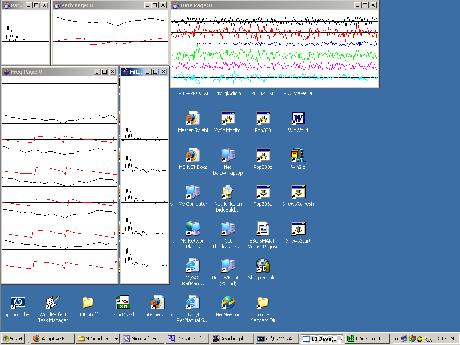
The graphic output
The program produces five graphs with three graphs in a row across the top of the screen and two graphs in a row below the top row as shown by the screen shot in Figure 1.
Figure 1 |
Description of the five graphs
A brief description of each of the five graphs, working from left to right, top to bottom, follows:
Multiple stacked pages
Graph 3, showing the time series data, consists of multiple pages stacked on top of one another. You can move the pages on the top of the stack to view the pages further down. The pages on the top of the stack represent the results produced early in the adaptive process while those further down represent the results produced later in the adaptive process.
(If you increase the number of iterations described later, graphs 4 and 5 will also consist of multiple pages stacked on top of one another.)
The six time series and their colors
The six time series that are plotted in Graph #3 are, from top to bottom in the colors indicated:
Impulse responses near the end of the run
Near the end of the run, the adaptive update process is disabled. The input data is set to zero for the remainder of the run except that on one occasion, an impulse is inserted into the white noise data. This makes it possible to see:
Ideally, the impulse response on the blue trace would be identical to the impulse response on the red trace, indicating that the adaptive filter perfectly matches the convolution filter that is applied to the white noise before it is added to the white signal. As you will see later, the match is not perfect but it is very close.
User input
There is no user input to this program. All parameter values are hard coded into the main method. To run the program with different parameters, modify the parameter values in the source code and recompile the program.
Program parameters
The important program parameters that you might want to modify for experimental purposes are:
Program testing
This program was tested using J2SE 5.0 and WinXP. J2SE 5.0 or later is required.
Before getting into the program details, I'm going to show you some experimental results.
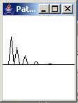
The acoustic path operator
The left panel in Figure 2 shows the convolution operator that was applied to the white noise to simulate the noise arriving at the location in the park where the concert is being held. When this convolution operator is applied to the white noise time series, the result is the sum of the primary time series plus four attenuated and time-delayed replicas of the time series. This is intended to simulate the summation of the original waterfall noise plus several echoes.
(Note that this convolution operator also inserts a time delay of several samples relative to its input.)
 |
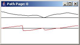 |
Figure 2 |
|
Complex frequency response
The right panel in Figure 2 shows the complex frequency response of the acoustic path operator. The top curve is the amplitude response and the bottom curve is the phase response.
As you can see this particular configuration of echoes results in a decidedly non-flat transfer function. The general saw tooth nature of the phase response indicates that there is an overall time delay in addition to the modification of the acoustic energy as a function of frequency.
The adaptive filter operator
The left panel in Figure 3 shows the development of the adaptive filter convolution operator from the beginning to the end of the run. Each of the individual graphs beginning at the top and going down the page shows the adaptive convolution operator at the end of every 400th iteration.
 |
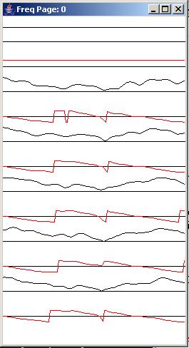 |
Figure 3 |
|
Ideally, the convolution operator in Figure 3 should converge to a shape that exactly matches the shape of the convolution operator shown in the left panel of Figure 2. As you can see, although the match isn't perfect, it is reasonably close at the bottom of Figure 3. The continuing random influence of the white signal would probably prevent a perfect solution from ever being achieved regardless of how long the adaptive process is allowed to run.
The complex frequency response
The right panel in Figure 3 shows the complex frequency response corresponding to each of the impulse responses in the left panel. As before, for each complex frequency response, the amplitude response is above the phase response.
The time series
The top panel in Figure 4 shows the six time series described earlier at the beginning of the run. The middle panel shows the same six traces in the time period immediately following the period shown in the top panel. The bottom panel shows the same six time series at the end of the run.
(Note that several panels of time series between the beginning and the end of the run were omitted for brevity.)
 |
 |
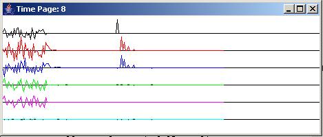 |
Figure 4 |
The white waterfall noise
As explained earlier, the black trace in Figure 4 shows the white waterfall noise that is transmitted to the adaptive engine via electrical cable without any influence from the acoustic path. This trace is used as an input to the adaptive process.
Signal plus modified waterfall noise
The red trace in Figure 4 shows the sum of the white signal and the output from the acoustic path operator shown in Figure 2. This trace is used as an input to the adaptive process.
Output from the adaptive filter
The blue trace in Figure 4 shows the output from the adaptive filter. The adaptive filter attempts to cause its output to match the output from the acoustic path operator so that when it is subtracted from the red trace, the result will be the pure signal. In other words, this is an estimate of the waterfall noise as modified by the acoustic path to the concert area.
The adaptive output error
The green trace in Figure 4 shows the error in the adaptive process. For this configuration of the adaptive engine, this is the trace that contains the signal with the noise having (hopefully) been removed.
The pure signal
As mentioned earlier, the violet trace in Figure 4 shows the original pure signal. This trace is not used in the adaptive process. Rather, it is provided here for visual comparison with the green trace that shows the adaptive process' estimate of the signal after the noise has been removed.
Estimate of the signal quality
Also as mentioned earlier, the turquoise trace in Figure 4 shows the arithmetic difference between the pure signal (violet) trace and the green trace containing the adaptive process' estimate of the signal. This trace is not used in the adaptive process. Rather, it is provided for a visual arithmetic comparison of the difference between the pure signal trace and the adaptive estimate of the signal. Ideally this trace will go to zero if the adaptive process is successful in totally eliminating the noise from the green trace.
The adaptive results
You can see the result of the adaptive process by comparing the traces from left to right in Figure 4. As you can see, the green error trace is a reasonably good replica of the violet signal trace by the end of the top panel, and is an excellent replica of the violet signal trace by the end of the middle panel. Thus, the noise is being almost totally suppressed from the red trace by the end of the middle panel.
The impulse responses
As explained earlier, the adaptive process is turned off and an impulse is injected into the black trace in the bottom panel of Figure 4. The impulse response of the acoustic path is shown by the red trace in the bottom panel. The impulse response of the final adaptive filter is shown by the blue trace in the bottom panel of Figure 4.
The objective of the adaptive process is to cause the impulse response of the adaptive filter to match the impulse response of the acoustic path. A visual comparison of the red and blue traces in the bottom panel of Figure 4 shows the extent to which this has been accomplished.
Now let's see some code.
The class named Adapt08
The beginning of the class named Adapt08 and the beginning of the main method are shown in Listing 1.
class Adapt08{
public static void main(String[] args){
//Default parameter values
double feedbackGain = 0.0001;
int numberIterations = 2001;
int filterLength = 26;//Must be >= 26 for plotting.
double noiseScale = 10;
double signalScale = 10;
|
Listing 1 declares and initializes some of the program parameters. To experiment with different values for the program parameters, change the values in Listing 1 and recompile the program.
The acoustic path operator
Listing 2 defines the impulse response of the path operator that simulates the acoustic path between the waterfall and the location in the park where the concert is being performed. (This impulse response is shown graphically in Figure 2.)
double[] pathOperator = {0.0,
0.0,
0.0,
1.0,
0.0,
0.64,
0.0,
0.0,
0.32768,
0.0,
0.0,
0.0,
0.1342176,
0.0,
0.0,
0.0,
0.0,
0.0439803,
0.0};
|
Note that the first three values in the impulse response have values of zero. This has the effect of inserting an overall time delay in the acoustic path. The value of 1.0 in the impulse response represents the first arrival of the acoustic waterfall noise at the concert location. The remaining non-zero values in the impulse response represent attenuated echoes that are further delayed in time relative to the first arrival.
To experiment with different acoustic path operators, change the values in Listing 2 and recompile the program. See if you can devise an acoustic path operator for which the adaptive algorithm will refuse to converge to a solution.
Invoke the method named process
Listing 3 instantiates an object of the Adapt08 class and invokes the process method on that object, passing the program parameters along with the acoustic path operator to the method.
new Adapt08().process(feedbackGain,
numberIterations,
filterLength,
noiseScale,
signalScale,
pathOperator);
}//end main
|
The process method
Listing 4 shows the beginning of the process method, including the code required to display the two graphs shown in Figure 2. This is the primary adaptive processing and plotting method for the program.
void process(double feedbackGain,
int numberIterations,
int filterLength,
double noiseScale,
double signalScale,
double[] pathOperator){
//The following array will be populated with the
// adaptive filter for display purposes.
double[] filter = null;
//Display the pathOperator
//First instantiate a plotting object.
PlotALot01 pathOperatorObj = new PlotALot01("Path",
(pathOperator.length * 4) + 8,148,70,4,0,0);
//Feed the data to the plotting object.
for(int cnt = 0;cnt < pathOperator.length;cnt++){
pathOperatorObj.feedData(40*pathOperator[cnt]);
}//end for loop
//Cause the graph to be displayed on the computer
// screen in the upper left corner.
pathOperatorObj.plotData(0,0);
//Now compute and plot the frequency response of the
// path
//Instantiate a plotting object for two channels of
// frequency response data. One channel is for
// the amplitude and the other channel is the phase.
PlotALot03 pathFreqPlotObj =
new PlotALot03("Path",264,148,35,2,0,0);
//Compute the frequency response and feed the results
// to the plotting object.
displayFreqResponse(pathOperator,pathFreqPlotObj,
128,0);
//Cause the frequency response data stored in the
// plotting object to be displayed on the screen in
// the top row of images.
pathFreqPlotObj.plotData(112,0);
|
All of the code shown in Listing 4 has been explained in earlier lessons referred to in the References section of this lesson. That explanation won't be repeated here.
Instantiate an adaptive engine object
Listing 5 instantiates an object that will be used to handle the adaptive behavior of the program.
AdaptEngine02 adapter = new AdaptEngine02(
filterLength,feedbackGain);
|
The class named AdaptEngine02 was explained in the lesson titled Adaptive Identification and Inverse Filtering using Java, and that explanation won't be repeated here.
Prepare for the iterative adaptive process
Listing 6 performs several additional steps that are necessary to prepare for the iterative adaptive process and plot the results of the adaptive process.
//Instantiate an array object that will be used as a
// delay line for the white noise data.
double[] rawData = new double[pathOperator.length];
//Instantiate a plotting object for six channels of
// time-series data.
PlotALot07 timePlotObj =
new PlotALot07("Time",468,198,25,2,0,0);
//Instantiate a plotting object for two channels of
// filter frequency response data. One channel is for
// the amplitude and the other channel is for the
// phase.
PlotALot03 freqPlotObj =
new PlotALot03("Freq",264,487,35,2,0,0);
//Instantiate a plotting object to display the filter
// impulse response at specific time intervals during
// the adaptive process.
PlotALot01 filterPlotObj = new PlotALot01("Filter",
(filterLength * 4) + 8,487,70,4,0,0);
//Declare and initialize working variables.
double output = 0;
double err = 0;
double target = 0;
double input = 0;
double whiteNoise = 0;
double whiteSignal = 0;
boolean adaptOn;
|
The code in Listing 6 is very similar to code that I have explained in previous lessons referred to in the References section of this lesson. I won't bore you by repeating those explanations here.
Perform the iterative adaptive process
Listing 7 shows the beginning of a for loop that is used to perform the specified number of iterations of the adaptive process.
for(int cnt = 0;cnt < numberIterations;cnt++){
adaptOn = true;
|
The variable named adaptOn
The variable named adaptOn is used to control whether or not the adapt method of the adaptive engine updates the filter coefficients when it is called. The filters are updated when this variable is true and are not updated when this variable is false. The value of this variable is maintained as true until near the end of the specified number of iterations. At that time, it is set to false to support the display of the impulse responses shown in the bottom panel of Figure 4.
(The adaptive process is disabled at that point in time to prevent the coefficients belonging to the adaptive filter from being modified while the impulse response of the adaptive filter is being displayed.)
Get white signal and noise values
Listing 8 gets and scales the next sample of white noise and white signal data from a random number generator. The white noise is used to simulate the waterfall noise. Before scaling by noiseScale and signalScale, the values are uniformly distributed from -1.0 to 1.0.
whiteNoise = noiseScale*(2*(Math.random() - 0.5));
whiteSignal = signalScale*(2*(Math.random() - 0.5));
|
Produce impulse responses near the end of the run
The code in Listing 9 sets the white noise and white signal values near the end of the run to zero and turns adaptation off by setting the value of adaptOn to false.
This code also inserts a single impulse near the end of the whiteNoise data that produces impulse responses for the acoustic path and for the adaptive filter.
The code in Listing 9 produces the impulse responses shown in the bottom panel of Figure 4.
//Set values to zero
if(cnt > (numberIterations - 5*filterLength)){
whiteNoise = 0;
whiteSignal = 0;
adaptOn = false;
}//end if
//Now insert an impulse at one specific location in
// the whiteNoise data.
if(cnt == numberIterations - 3*filterLength){
whiteNoise = 2 * noiseScale;
}//end if
|
Convolve waterfall noise with acoustic path operator
Listing 10 convolves the waterfall noise with the acoustic path operator to produce an estimate of the waterfall noise as it would sound at the location in the park where the concert is being performed.
//Insert the white noise data into the delay line
// that will be used to convolve the white noise
// with the path operator.
flowLine(rawData,whiteNoise);
//Apply the path operator to the white noise data.
double pathNoise =
reverseDotProduct(rawData,pathOperator);
|
Code similar to that shown in Listing 10 has been explained in earlier lessons referred to in the References section of this lesson. Therefore, I won't repeat that explanation here.
Perform the adaptive process
The code in Listing 11 performs the adaptive process for one iteration of the for loop that began in Listing 7.
Listing 11 begins by declaring a variable that will be populated with a reference to an object containing the results returned by the adapt method of the adaptive engine.
//Declare a variable that will be populated with the
// results returned by the adapt method of the
// adaptive engine.
AdaptiveResult result = null;
//Establish the appropriate input values for an
// adaptive noise cancellation filter and perform the
// adaptive update.
input = whiteNoise;
target = pathNoise + whiteSignal;
result = adapter.adapt(input,target,adaptOn);
|
The two boldface statements in Listing 11 make this program unique and different relative to the other programs explained in the earlier lessons referred to in the References section of this lesson.
The general-purpose adaptive engine
When I developed the general purpose adaptive engine in the lesson titled A General-Purpose LMS Adaptive Engine in Java, I explained:
"In this lesson, I will present and explain a general-purpose LMS adaptive engine written in Java that can be used to solve a wide variety of adaptive problems."
The adaptive engine receives two input time series and produces two output time series. The engine can be used to solve different problems by carefully selecting the two input time series and order in which they are provided to the adaptive engine.
The configuration for adaptive noise cancellation
In Listing 11, the whiteNoise is provided to simulate the waterfall noise and is inserted into the adaptive filter as shown by the Reference Signal in the block diagram.
The target in Listing 11 is constructed by adding the pathNoise to the whiteSignal. This addition corresponds to the dotted circle with the plus sign at the top of the block diagram.
The value of whiteSignal in Listing 11 corresponds to the Primary Signal in the block diagram.
The value of the pathNoise in Listing 11 corresponds to the output from the dotted box containing the question mark in the block diagram.
The target in Listing 11 corresponds to d(n) in the block diagram.
The output from the adaptive filter is subtracted from the target value to produce the error. The error is used in a feedback loop to adjust the adaptive filter coefficients as shown in the block diagram.
For this configuration, the error is also the primary output shown by the green trace in Figure 4.
Finish an adaptive iteration
Listing 12 shows the remaining code in the for loop that began in Listing 7.
//Get and save adaptive results for plotting and
// spectral analysis
output = result.output;
err = result.err;
filter = result.filterArray;
//Feed the time series data to the plotting object.
timePlotObj.feedData(input,target,output,-err,
whiteSignal,err + whiteSignal);
//Compute and plot summary results at the end of
// every 400th iteration.
if(cnt%400 == 0){
displayFreqResponse(filter,freqPlotObj,
128,filter.length - 1);
//Display the filter impulse response coefficient
// values. The adaptive engine returns the filter
// with the time axis reversed relative to the
// conventional display of an impulse response.
// Therefore, it is necessary to display it in
// reverse order.
for(int ctr = 0;ctr < filter.length;ctr++){
filterPlotObj.feedData(
40*filter[filter.length - 1 - ctr]);
}//end for loop
}//End display of frequency response and filter
}//End for loop
|
All of the code in Listing 12 is very similar to code that I have explained in earlier lessons referred to by the References section of this lesson. Therefore, I won't repeat that explanation here.
Complete the process method
Listing 13 shows the remaining code in the process method.
//Cause the data stored in the plotting objects to be
// plotted.
timePlotObj.plotData(376,0);//Top of screen
freqPlotObj.plotData(0,148);//Left side of screen
filterPlotObj.plotData(265,148);
}//end process method
|
Shall I say it one more time? All of the code in Listing 13 is very similar to code that I have explained in earlier lessons referred to by the References section of this lesson. Therefore, I won't repeat that explanation here.
Further, the remaining methods belonging to the Adapt08 class are similar to methods that I have explained in earlier lessons, so I won't discuss those methods here. You can view the code for the class named Adapt08 in its entirety in Listing 14 near the end of this lesson.
I encourage you to copy the code for the class named Adapt08 from the section titled Complete Program Listings. Compile and execute the program. Experiment with the code. Make changes to the code, recompile, execute, and observe the results of your changes.
Modify the program parameters and the path operator and see if you can explain the results of those modifications.
See if you can create a path operator for which the adaptive process refuses to converge to a solution.
Experiment with different values for feedback Gain. What happens if you use a large value for feedbackGain? What happens if you use a very small value for feedbackGain? What happens if you use a negative value for feedbackGain? Can you explain the results that you experience?
While experimenting with the feedbackGain, you might also want to experiment with the program parameter named numberIterations. See if you can explain the results for small, medium, and large values for this parameter.
Other classes required
In addition to the classes named Adapt08, you will need access to the following classes. The source code for these classes can be found in the lessons indicated.
In this lesson, I showed you how to use a general-purpose LMS adaptive engine to write a Java program that illustrates the use of adaptive filtering for Noise Cancellation.
Adaptive filtering is commonly used for the following four scenarios:
A previous lesson titled Adaptive Identification and Inverse Filtering using Java explained how to write Java programs to illustrate the first two scenarios in the above list. This lesson explains how to write a Java program that illustrates the use of adaptive filtering for the third scenario: Noise Cancellation.
I plan to publish a lesson in the near future that explains and provides examples of Prediction using adaptive filtering.
In preparation for understanding the material in this lesson, I recommend that you study the material in the following previously-published lessons:
Links to the lessons in the above list are available at Digital Signal Processing-DSP.
A complete listings of the class discussed in this lesson is shown in Listing 14 below.
/*File Adapt08.java
Copyright 2005, R.G.Baldwin
The purpose of this program is to illustrate an adaptive
noise cancellation system.
See the following URL for a description and a block
diagram of an adaptive noise cancellation system.
http://www.owlnet.rice.edu/~ryanking/elec431/intro.html
This program requires the following classes:
Adapt08.class
AdaptEngine02.class
AdaptiveResult.class
ForwardRealToComplex01.class
PlotALot01.class
PlotALot03.class
PlotALot07.class
This program uses the adaptive engine named AdaptEngine02
to adaptively develop a filter. One of the inputs to the
adaptive engine is the sum of signal plus noise. The
other input to the adaptive engine is noise that is
different from, but which is correlated to the noise that
is added to the signal. The adaptive engine develops a
filter that removes the noise from the signal plus noise
data producing an output consisting of almost pure
signal.
The signal and the original noise are derived from a
random number generator. Therefore, they are both
essentially white. The signal is not correlated with the
noise. Before scaling, the values obtained from the
random number generator are uniformly distributed from
-1.0 to +1.0.
The white noise is processed through a convolution
filter before adding it to the signal. The convolution
filter is designed to simulate the effect of acoustic
energy being emitted at one point in space and being
modified through the addition of several time-delayed and
attenuated echoes before being received at another point
in space. This results in constructive and destructive
interference such that the noise that is added to the
signal is no longer white. However, it is still
correlated with the original white noise.
The program produces five graphs with three graphs in a
row across the top of the screen and two graphs in a row
below the top row.
The following is a brief description of each of the five
graphs, working from left to right, top to bottom.
1. The impulse response of the convolution filter that is
applied to the white noise before it is added to the
white signal.
2. The amplitude and phase response of the convolution
filter that is applied to the white noise before it is
added to the white signal.
3. Six time series that illustrate the time behavior of
the adaptive process.
4. The amplitude and phase response of the adaptive
filter at the end of every 400th iteration.
5. The impulse response of the adaptive filter at the end
of every 400th adaptive iteration.
Graph 3 consists of multiple pages stacked on top
of one another. Move the pages on the top of the stack to
view the pages further down. The pages on the top of the
stack represent the results produced early in the adaptive
process while those further down represent the results
produced later in the adaptive process. If you increase
the number of iterations described later, graphs 4 and 5
will also consist of multiple pages stacked on top of one
another.
The six time series that are plotted are, from top to
bottom in the colors indicated:
1. (Black) Input to the adaptive filter. This is the
white noise.
2. (Red) Target for the adaptive process. This is the
signal plus noise.
3. (Blue) Output from the adaptive filter.
4. (Green) Error computed within the adaptive process.
In this case, the error trace is actually the trace that
contains the signal with the noise removed. In other
words, the blue trace is an estimate of the noise and the
green trace is the difference between the red trace and
the blue trace.
5. (Violet) The original pure signal. This trace is
provided for visual comparison with the green signal trace.
6. (Turquoise) The arithmetic difference between the
pure signal trace (violet) and the green trace containing
the adaptive process's estimate of the signal. This
trace is provided for an arithmetic comparison of the
pure signal trace and the adaptive estimate of the signal.
Ideally this trace will go to zero if the adaptive process
is successful in totally eliminating the noise from the
green trace.
Near the end of the run, the adaptive update process is
disabled. The input data is set to zero for the remainder
of the run except that on one occasion, an impulse is
inserted into the white noise data. This makes it
possible to see:
1. The impulse response of the convolution filter that
is applied to the white noise before it is added to the
white signal.
2. The impulse response of the final adaptive filter.
There is no user input to this program. All parameters are
hard coded into the main method. To run the program with
different parameters, modify the parameters and recompile
the program.
The program parameters are:
feedbackGain: The gain factor that is used in the feedback
loop to adjust the coefficient values in the adaptive
filter.
numberIterations: This is the number of iterations that the
program executes before stopping and displaying all of the
graphic results.
filterLength: This is the number of coefficients in the
adaptive filter. Must be at least 26. If you change it
to a value that is less than 26, the plot of the impulse
responses of the adaptive filter will not be properly
aligned.
noiseScale: The scale factor that is applied to the values
that are extracted from the random number generator and
used as white noise.
signalScale: The scale factor that is applied to the
values that are extracted from the random number generator
and used as white signal.
pathOperator: Areference to an array of type double[]
containing the coefficients of the convolution filter that
is applied to the white noise before it is added to the
white signal.
Tested using J2SE 5.0 and WinXP. J2SE 5.0 or later is
required.
**********************************************************/
import static java.lang.Math.*;//J2SE 5.0 req
class Adapt08{
public static void main(String[] args){
//Default parameter values
double feedbackGain = 0.0001;
int numberIterations = 2001;
int filterLength = 26;//Must be >= 26 for plotting.
double noiseScale = 10;
double signalScale = 10;
//Define the path impulse response as a simulation of
// an acoustic signal with time-delayed echoes.
double[] pathOperator = {0.0,
0.0,
0.0,
1.0,
0.0,
0.64,
0.0,
0.0,
0.32768,
0.0,
0.0,
0.0,
0.1342176,
0.0,
0.0,
0.0,
0.0,
0.0439803,
0.0};
//Instantiate a new object of the Adapt08 class
// and invoke the method named process on that object.
new Adapt08().process(feedbackGain,
numberIterations,
filterLength,
noiseScale,
signalScale,
pathOperator);
}//end main
//-----------------------------------------------------//
//This is the primary adaptive processing and plotting
// method for the program.
void process(double feedbackGain,
int numberIterations,
int filterLength,
double noiseScale,
double signalScale,
double[] pathOperator){
//The following array will be populated with the
// adaptive filter for display purposes.
double[] filter = null;
//Display the pathOperator
//First instantiate a plotting object.
PlotALot01 pathOperatorObj = new PlotALot01("Path",
(pathOperator.length * 4) + 8,148,70,4,0,0);
//Feed the data to the plotting object.
for(int cnt = 0;cnt < pathOperator.length;cnt++){
pathOperatorObj.feedData(40*pathOperator[cnt]);
}//end for loop
//Cause the graph to be displayed on the computer
// screen in the upper left corner.
pathOperatorObj.plotData(0,0);
//Now compute and plot the frequency response of the
// path
//Instantiate a plotting object for two channels of
// frequency response data. One channel is for
// the amplitude and the other channel is the phase.
PlotALot03 pathFreqPlotObj =
new PlotALot03("Path",264,148,35,2,0,0);
//Compute the frequency response and feed the results
// to the plotting object.
displayFreqResponse(pathOperator,pathFreqPlotObj,
128,0);
//Cause the frequency response data stored in the
// plotting object to be displayed on the screen in
// the top row of images.
pathFreqPlotObj.plotData(112,0);
//Instantiate an object to handle the adaptive behavior
// of the program.
AdaptEngine02 adapter = new AdaptEngine02(
filterLength,feedbackGain);
//Instantiate an array object that will be used as a
// delay line for the white noise data.
double[] rawData = new double[pathOperator.length];
//Instantiate a plotting object for six channels of
// time-series data.
PlotALot07 timePlotObj =
new PlotALot07("Time",468,198,25,2,0,0);
//Instantiate a plotting object for two channels of
// filter frequency response data. One channel is for
// the amplitude and the other channel is for the
// phase.
PlotALot03 freqPlotObj =
new PlotALot03("Freq",264,487,35,2,0,0);
//Instantiate a plotting object to display the filter
// impulse response at specific time intervals during
// the adaptive process.
PlotALot01 filterPlotObj = new PlotALot01("Filter",
(filterLength * 4) + 8,487,70,4,0,0);
//Declare and initialize working variables.
double output = 0;
double err = 0;
double target = 0;
double input = 0;
double whiteNoise = 0;
double whiteSignal = 0;
boolean adaptOn;
//Perform the specified number of iterations.
for(int cnt = 0;cnt < numberIterations;cnt++){
//The following variable is used to control whether
// or not the adapt method of the adaptive engine
// updates the filter coefficients when it is called.
// The filters are updated when this variable is
// true and are not updated when this variable is
// false.
adaptOn = true;
//Get and scale the next sample of white noise and
// white signal data from a random number generator.
// Before scaling by noiseScale and signalScale, the
// values are uniformly distributed from -1.0 to 1.0.
whiteNoise = noiseScale*(2*(Math.random() - 0.5));
whiteSignal = signalScale*(2*(Math.random() - 0.5));
//Set white noise and white signal values near the
// end of the run to zero and turn adaptation off.
// Insert an impulse near the end of the whiteNoise
// data that will produce impulse responses for the
// path and for the adaptive filter.
//Set values to zero.
if(cnt > (numberIterations - 5*filterLength)){
whiteNoise = 0;
whiteSignal = 0;
adaptOn = false;
}//end if
//Now insert an impulse at one specific location in
// the whiteNoise data.
if(cnt == numberIterations - 3*filterLength){
whiteNoise = 2 * noiseScale;
}//end if
//Insert the white noise data into the delay line
// that will be used to convolve the white noise
// with the path operator.
flowLine(rawData,whiteNoise);
//Apply the path operator to the white noise data.
double pathNoise =
reverseDotProduct(rawData,pathOperator);
//Declare a variable that will be populated with the
// results returned by the adapt method of the
// adaptive engine.
AdaptiveResult result = null;
//Establish the appropriate input values for an
// adaptive noise cancellation filter and perform the
// adaptive update.
input = whiteNoise;
target = pathNoise + whiteSignal;
result = adapter.adapt(input,target,adaptOn);
//Get and save adaptive results for plotting and
// spectral analysis
output = result.output;
err = result.err;
filter = result.filterArray;
//Feed the time series data to the plotting object.
timePlotObj.feedData(input,target,output,-err,
whiteSignal,err + whiteSignal);
//Compute and plot summary results at the end of
// every 400th iteration.
if(cnt%400 == 0){
displayFreqResponse(filter,freqPlotObj,
128,filter.length - 1);
//Display the filter impulse response coefficient
// values. The adaptive engine returns the filter
// with the time axis reversed relative to the
// conventional display of an impulse response.
// Therefore, it is necessary to display it in
// reverse order.
for(int ctr = 0;ctr < filter.length;ctr++){
filterPlotObj.feedData(
40*filter[filter.length - 1 - ctr]);
}//end for loop
}//End display of frequency response and filter
}//End for loop,
//Cause the data stored in the plotting objects to be
// plotted.
timePlotObj.plotData(376,0);//Top of screen
freqPlotObj.plotData(0,148);//Left side of screen
filterPlotObj.plotData(265,148);
}//end process method
//-----------------------------------------------------//
//This method simulates a tapped delay line. It receives
// a reference to an array and a value. It discards the
// value at index 0 of the array, moves all the other
// values by one element toward 0, and inserts the new
// value at the top of the array.
void flowLine(double[] line,double val){
for(int cnt = 0;cnt < (line.length - 1);cnt++){
line[cnt] = line[cnt+1];
}//end for loop
line[line.length - 1] = val;
}//end flowLine
//-----------------------------------------------------//
void displayFreqResponse(
double[] filter,PlotALot03 plot,int len,int zeroTime){
//Create the arrays required by the Fourier Transform.
double[] timeDataIn = new double[len];
double[] realSpect = new double[len];
double[] imagSpect = new double[len];
double[] angle = new double[len];
double[] magnitude = new double[len];
//Copy the filter into the timeDataIn array
System.arraycopy(filter,0,timeDataIn,0,filter.length);
//Compute DFT of the filter from zero to the folding
// frequency and save it in the output arrays.
ForwardRealToComplex01.transform(timeDataIn,
realSpect,
imagSpect,
angle,
magnitude,
zeroTime,
0.0,
0.5);
//Note that the conversion to decibels has been
// disabled. You can re-enable the conversion by
// removing the comment indicators.
/*
//Display the magnitude data. Convert to normalized
// decibels first.
//Eliminate or change any values that are incompatible
// with log10 method.
for(int cnt = 0;cnt < magnitude.length;cnt++){
if((magnitude[cnt] == Double.NaN) ||
(magnitude[cnt] <= 0)){
//Replace the magnitude by a very small positive
// value.
magnitude[cnt] = 0.0000001;
}else if(magnitude[cnt] == Double.POSITIVE_INFINITY){
//Replace the magnitude by a very large positive
// value.
magnitude[cnt] = 9999999999.0;
}//end else if
}//end for loop
//Now convert magnitude data to log base 10
for(int cnt = 0;cnt < magnitude.length;cnt++){
magnitude[cnt] = log10(magnitude[cnt]);
}//end for loop
*/
//Find the absolute peak value. Begin with a negative
// peak value with a large magnitude and replace it
// with the largest magnitude value.
double peak = -9999999999.0;
for(int cnt = 0;cnt < magnitude.length;cnt++){
if(peak < abs(magnitude[cnt])){
peak = abs(magnitude[cnt]);
}//end if
}//end for loop
//Normalize to 20 times the peak value
for(int cnt = 0;cnt < magnitude.length;cnt++){
magnitude[cnt] = 20*magnitude[cnt]/peak;
}//end for loop
//Now feed the normalized data to the plotting
// object.
for(int cnt = 0;cnt < magnitude.length;cnt++){
plot.feedData(magnitude[cnt],angle[cnt]/20);
}//end for loop
}//end displayFreqResponse
//-----------------------------------------------------//
//This method receives two arrays and treats each array
// as a vector. The two arrays must have the same length.
// The program reverses the order of one of the vectors
// and returns the vector dot product of the two vectors.
double reverseDotProduct(double[] v1,double[] v2){
if(v1.length != v2.length){
System.out.println("reverseDotProduct");
System.out.println("Vectors must be same length.");
System.out.println("Terminating program");
System.exit(0);
}//end if
double result = 0;
for(int cnt = 0;cnt < v1.length;cnt++){
result += v1[cnt] * v2[v1.length - cnt - 1];
}//end for loop
return result;
}//end reverseDotProduct
//-----------------------------------------------------//
}//end class Adapt08
|
Copyright 2006, Richard G. Baldwin. Reproduction in whole or in part in any form or medium without express written permission from Richard Baldwin is prohibited.
Richard has participated in numerous consulting projects and he frequently provides onsite training at the high-tech companies located in and around Austin, Texas. He is the author of Baldwin's Programming Tutorials, which have gained a worldwide following among experienced and aspiring programmers. He has also published articles in JavaPro magazine.
In addition to his programming expertise, Richard has many years of practical experience in Digital Signal Processing (DSP). His first job after he earned his Bachelor's degree was doing DSP in the Seismic Research Department of Texas Instruments. (TI is still a world leader in DSP.) In the following years, he applied his programming and DSP expertise to other interesting areas including sonar and underwater acoustics.
Richard holds an MSEE degree from Southern Methodist University and has many years of experience in the application of computer technology to real-world problems.
Keywords
Java adaptive filtering convolution filter frequency spectrum LMS amplitude
phase time-delay linear DSP impulse decibel log10 DFT transform bandwidth signal
noise real-time dot-product vector time-series prediction identification inverse
noise cancellation
-end-