Figure 1
Published: February 7, 2006
by Richard G. Baldwin
Java Programming Notes # 2358
DSP and adaptive filtering
With the decrease in cost and the increase in speed of digital devices, Digital Signal Processing (DSP) is showing up in everything from cell phones to hearing aids to rock concerts. Many applications of DSP are static. That is, the characteristics of the digital processor don't change with time or circumstances. However, a particularly interesting branch of DSP is adaptive filtering. This is a scenario where the characteristics of the digital processor change with time, circumstances, or both.
Fifth in a series
This is the fifth lesson in a series designed to teach you about adaptive filtering in Java. The first lesson, titled Adaptive Filtering in Java, Getting Started, introduced you to the topic by showing you how to write a Java program to adaptively design a time-delay convolution filter with a flat amplitude response and a linear phase response using an LMS adaptive algorithm.
A general-purpose adaptive engine
The third lesson in the series, titled A General-Purpose LMS Adaptive Engine in Java, presented and explained a general-purpose LMS adaptive engine written in Java. That engine can be used to solve a wide variety of adaptive problems.
An adaptive line tracker
The previous lesson titled An Adaptive Line Tracker in Java showed you how to use the general-purpose LMS adaptive engine to develop an adaptive spectral line tracker in Java. At the end of that lesson, I promised that future lessons would teach you about the following four general topics in adaptive filtering:
This lesson presents and explains a program named Adapt07, which demonstrates the use of adaptive filtering for System Identification and Inverse System Identification. Future lessons will deal with the other two items in the above list.
Viewing tip
You may find it useful to open another copy of this lesson in a separate browser window. That will make it easier for you to scroll back and forth among the different listings and figures while you are reading about them.
Supplementary material
I recommend that you also study the other lessons in my extensive collection of online Java tutorials. You will find those lessons published at Gamelan.com. However, as of the date of this writing, Gamelan doesn't maintain a consolidated index of my Java tutorial lessons, and sometimes they are difficult to locate there. You will find a consolidated index at www.DickBaldwin.com.
In preparation for understanding the material in this lesson, I recommend that you also study the lessons identified in the References section of this document.
What is system identification and system inversion?
Let me try to explain these terms using an example with which most of us are familiar. At some time in your life, you have probably attended a gathering in a venue such as a stadium or an auditorium and you came away with the general conclusion that the acoustics were bad.
What is meant by the acoustics are bad?
When you are located in different seats in such a venue, the acoustics may be good or they may be bad depending on where you are seated. For example, in some seats, you may be able to understand the announcer very clearly. In other seats, echoes, absorption, and other acoustic problems may make the announcer's voice very difficult to understand.
(Or, it may be that the electronic audio system is of poor quality causing the acoustics to be bad in all the seats.)
An acoustic system
We can think of the acoustic and electronic path between the announcer's vocal chords and your ears as an acoustic system. That system can be characterized by a complex frequency response and a corresponding impulse response.
A hypothetical measuring device
Assume for example that you have a portable device on which you can record two tracks of electronic data. Assume that you move this device around the auditorium recording what you hear at different locations. Assume that on one track you record the electronic signal produced by the announcer's microphone. Assume that on the other track you record the electronic output produced by a portable microphone that you carry with you.
The system transfer function
There are a variety of techniques available for analyzing the two recorded electronic signals in order to determine the complex transfer function resulting from the many electronic and physical components between those two points in the system.
Electronic transfer problems
For example, the amplifier and the loud speakers up on the stage may or may not produce a high-quality representation of the electronic output from the announcer's microphone. For example, the amplitude response of the amplifier and the speakers may not be flat across the desired range of frequencies. In addition, they may introduce phase distortion at certain frequencies causing words to sound distorted.
Physical transfer problems
Items such as drapes and carpets in the auditorium may absorb acoustic energy at certain audio frequencies preventing the acoustic energy at those frequencies from reaching your ears.
Various surfaces in the auditorium may produce echoes causing you to hear the same thing more than once. Interference patterns produced by the intersecting waves of acoustic echo energy may cause acoustic energy at certain frequencies and certain locations to interact constructively or destructively. This can cause the sound at some frequencies to be too loud and the sound at other frequencies to be too soft.
The overall system transfer function
All of these factors taken together result in a complex transfer function between the electronic signal produced by the announcer's microphone and the electronic signal produced by your portable microphone in a different location in the auditorium. One way to characterize this transfer function is through the development of an adaptive identification filter.
An inverse filter
Once you have characterized the system transfer function, it may be possible to design an inverse digital filter than will compensate for many of the problems in the system transfer function, causing the combined response of the system transfer function and the inverse filter to have a nearly flat amplitude response and a nearly flat (or at least linear) phase response.
Adaptive filter design provides one approach to designing such an inverse filter. (There are other approaches available as well.) When adaptive filter design is used to design the inverse filter, it is not necessary to first characterize the transfer function and then to design an inverse filter as two separate operations. Rather, those two steps can be combined to produce a single result, which is the adaptive inverse filter.
Applicable to many different areas
Although I have described this process using only one scenario, these techniques are applicable to a variety of different technical areas ranging from telephone line equalization to rock concerts.
Other references
There are many good references to adaptive filtering available on the web, which you can locate using Google. Two of the references that I recommend are located here and here. I will be referring to some of the images contained on those web pages in the discussion that follows.
The program named Adapt07
The purpose of this program is to illustrate adaptive identification and adaptive inverse filtering.
This program requires the following classes:
With the exception of the first two items in the above list, I have presented and explained the source code for each of the classes in the above list in previous lessons. You will find references to those earlier lessons in the References section of this document.
The source code for the class named Adapt07 can be viewed in its entirety in Listing 17. The source code for the class named AdaptEngine02 can be viewed in Listing 18.
The class named AdaptEngine02
This program uses the adaptive engine named AdaptEngine02 to adaptively develop a filter. Depending on user input, the resulting filter is designed to be either an identification filter or an inverse filter.
The class named AdaptEngine02 is a simple upgrade to the class named AdaptEngine01 that was explained in earlier programs. This upgrade makes it possible for the user to pass a boolean parameter to the adapt method of the engine to either enable or disable the adaptive update of the filter coefficients. Because of the similarity of the two classes, I won't provide a detailed explanation of the class named AdaptEngine02 in this lesson.
User options
When the user opts for an identification filter, the adaptive process attempts to replicate the impulse response of a path through which wideband test data are flowing. When the user opts for an inverse filter, the adaptive process attempts to develop a filter that is the inverse of the impulse response of a path through which wideband test data are flowing.
Test cases
User-selectable test cases are provided for six different path scenarios. The user may develop an identification filter or an inverse filter for any of the six cases.
Graphic output
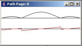
If the user opts for an identification filter, five separate graphs are produced. If the user opts for an inverse filter, six separate graphs are produced. The graphs appear on the screen in two rows with three graphs in each row as shown in Figure 1.
Figure 1 |
Description of the graphs
The following is a brief description of each of the six graphs, working from left to right, top to bottom.
Graphs with multiple pages
Graphs 3, 4, and 5 consist of multiple pages stacked on top of one another. You can move the pages on the top of the stack to view the pages further down. The pages on the top of the stack represent the results produced early in the adaptive process while those further down represent the results produced later in the adaptive process.
The time series
The four time series that are plotted in the third graph in the top row are, from top to bottom in the colors indicated:
Near the end of the run, the adaptive update process is disabled. The input data is set to zero for the remainder of the run except that on two subsequent occasions, an impulse is inserted into the data. This causes several interesting impulse responses to appear on the last page of the time-series plot.
The impulse responses
By running the same path twice, once in identification filter mode and once in inverse filter mode, the insertion of these impulses makes it possible to see:
Wideband test data
In operation, the program generates wideband test data produced by a random number generator and convolves it with a specified path impulse response to simulate the effect of the path on the test data. The original wideband test data and the path output data are both presented to the adaptive engine. The order in which the two are presented to the adaptive engine determines whether the adaptive engine will develop an identification filter or an inverse filter.
When the original wideband test data is presented as the data to be filtered within the adaptive engine and the path output is presented as the adaptive target, the adaptive process attempts to develop an adaptive filter that replicates the impulse response of the path. To help explain this, I am going to refer to the picture that you will find at The MathWorks web site.
(While you are there, it would also be a good idea for you to read what they have to say about adaptive filtering.)
Correspondence between my terms and the picture
The following paragraphs explain the correspondence between the terms that I use in this lesson and the terms used by the author of the picture. These relationships apply to the development of an identification filter. (I will address the relationships for an inverse filter a little later.)
The box labeled Unknown System in the picture is what I will refer to in this lesson as the path. The signal that the picture refers to as x(k), (which feeds both the adaptive filter and the path) is what I will refer to as wideband test data.
The signal that the picture refers to as d(k) is what I will refer to as the target. The signal that the picture refers to as e(k) is what I will refer to as the error.
Finally, everything inside the gray box in the picture corresponds to the adaptive engine in this lesson. The box labeled Adaptive Filter in the picture is what I will also refer to as the adaptive filter. It resides inside the adaptive engine.
Adaptive Filter and Unknown System are in parallel
As you can see from the picture, the wideband test data, or x(k) feeds into both the adaptive filter and the path. The target or d(k) feeds into the adaptive engine where it is combined algebraically with the output from the adaptive filter to produce the error or e(k).
(At this point, I have a small quarrel with the picture. The error should be processed through a multiplicative gain factor, feedbackGain, and used to adjust the filter coefficients. That isn't as obvious as it could be in the picture.)
Attempts to drive the error to zero
In any event, an LMS adaptive algorithm is used to adjust the coefficients in the adaptive filter in an attempt to drive the error to zero. When this is accomplished, the characteristics of the adaptive filter match the characteristics of the path. The adaptive filter then becomes an identification filter in that it identifies the characteristics of the Unknown System or the path.
When the two input time series that feed the adaptive engine are reversed, such that the path output is fed to the adaptive filter and the wideband test data is fed as the target, the adaptive process attempts to develop an adaptive filter that is the inverse of the impulse response of the path. To help explain this, I am going to refer to another picture that you will find at The MathWorks web site.
Correspondence between my terms and the other picture
The following paragraphs explain the correspondence between the terms that I will use in this lesson and the terms used by the author of the picture. These relationships apply to the development of an inverse filter in this lesson.
As before, the box in the picture labeled Unknown System is what I will refer to as the path. Everything inside the gray box in the picture is what I will refer to as the adaptive engine.
The signal that is referred to as s(k) in the picture is what I will refer to in this lesson as wideband test data. As you can see, after an appropriate delay, this signal also feeds the adaptive engine as the target or d(k).
As you can also see in the picture, the path output or x(k) feeds the adaptive filter in the adaptive engine. The output from the adaptive filter, y(k) is used to form the error e(k). In this picture, it is clear that the error is fed back and used to adjust the coefficients in the adaptive filter.
(However, even this picture is missing the feedbackGain factor.)
The path and the adaptive filter are in series
As in the previous case, the LMS adaptive algorithm adjusts the values of the filter coefficients in an attempt to drive the error to zero. When this is accomplished, the output from the adaptive filter replicates the wideband test data.
The only way that this can happen is for the characteristics of the adaptive filter to compensate for (cancel out) the characteristics of the path or the Unknown System. When one filter can be placed in series with another filter causing the combination of the two filters to be as if there were no filter in the system at all, one of those filters is known as the inverse of the other. This is sort of like the following arithmetic expression where 1/4 is the inverse of 4.
15 * (4 * (1/4)) = 15
Multiplying a value by 4 and then multiplying again by 1/4 is just like not multiplying at all (or multiplying by 1).
User input
User input is provided by five command-line parameters. If no command-line parameters are provided, default parameters are used. The command-line parameters are:
The minimum filter length
The minimum filter length of 26 has to do with plotting alignment issues and has nothing to do with the adaptive process. (See a description of the alignment issues in earlier lessons referred to in the References section of this document).
Six path scenarios are built into the code. The six path scenarios can be generally described as follows:
Program testing
The program was tested using J2SE 5.0 and WinXP. J2SE 5.0 or later is required.
Before getting into the program details, I'm going to show you some experimental results for three of the six path scenarios that are built into the program.
A low-pass filter with a short time constant
I will begin with the first scenario in the above list. I will also begin by developing an identification filter for this path scenario.
(This is the default case if you run the program without providing command-line parameters.)
The input parameters for this case are shown in Figure 2.
Input values were not provided.
Using following default values:
feedbackGain: 1.0E-4
numberIterations: 2001
filterLength: 26
testCase: 1
identification: true
Figure 2 |
The path characteristics
Let's begin by characterizing the path for this case. As you will see later when we examine the code, the coefficients in the impulse response that characterize this path are shown in Figure 3.
    double[] pathA = {1.0,
                      0.5,
                      0.25,
                      0.125,
                      0.0625,
                      0.03125,
                      0.015625,
                      0.0};
Figure 3 |
Those of you who are familiar with such things will recognize this as an impulse response with an inverse exponential decay, truncated to zero after seven filter coefficients.
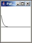
The impulse and frequency response of the path
This impulse response of the path is shown in graphic format in the left panel of Figure 4.
 |
 |
Figure 4 |
|
The right panel of Figure 4 shows the amplitude and phase response of this impulse response from zero to the Nyquist folding frequency. The black curve at the top of the panel is the amplitude response. The red line in the bottom of the panel is the phase response.
A low-pass filter
As you can see, this path characteristic tends to pass low-frequency signals and to suppress high-frequency signals.
(As I recall from my early days in the analog world, this is the digital equivalent of the response of a passive RC filter with an attenuation rate of six decibels per octave to the right of the corner frequency.)
The adaptive time series
The top panel in Figure 5 shows the adaptive time series at the beginning of the run. The bottom panel shows the time series at the end of the run.
 |
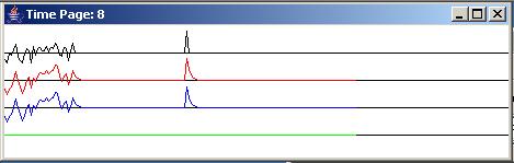 |
Figure 5 |
Description of the traces
The top (black) trace shows the wideband test data that is fed into the adaptive filter. The second (red) trace shows the path output data, which forms the adaptive target for the development of the identification filter. In other words, the red trace shows the result of applying the path impulse response shown in Figure 4 to the wideband test data shown by the black trace in Figure 5.
(A practiced eye can discern that the red trace is richer in low-frequency energy and leaner in high-frequency energy than the black trace.)
The adaptive filter output
The blue trace is the output from the adaptive filter. Initially, the output from the filter is zero because all of the coefficients are initialized to values of zero. However as time progresses from left to right in the top panel of Figure 5, we start to see some output from the adaptive filter.
The error trace
The error, shown by the green trace in Figure 5, is the difference between the red target trace and the blue adaptive filter output trace. Initially the error looks just like the red target trace in the top panel of Figure 5. However, as time progresses from left to right, the blue output trace begins to gain strength and the error trace begins to be reduced in amplitude.
Somewhat later in time
Finally, after about 2000 adaptive iterations (see the numberIterations parameter in Figure 2) we arrive at the bottom panel in Figure 5. By this point in time, the adaptive filter coefficients have been adjusted to drive the green error trace to zero. This was accomplished by causing the blue adaptive filter output trace to replicate the red target trace. At this point, the adaptive filter is a replica of the path, and the unknown characteristics of the path have been identified. Stated differently, those characteristics have been captured in a digital filter than can be easily analyzed.
Some impulse responses
As I explained earlier, near the end of the run, the adaptive update process is disabled and a single impulse is inserted into the wideband test data shown by the black trace in Figure 5.
(An impulse in a sampled-data system is a single non-zero value surrounded by values of zero.)
This impulse is filtered by the path characteristics, producing the output shown by the red trace, and is also filtered by the adaptive filter, producing the output shown by the blue trace. As you can see, the adaptive filter has been adjusted such that the impulse response of the adaptive filter is a very good replica of the impulse response of the path. Both impulse responses match the impulse response shown in Figure 4.
Adaptive progression
The left and right panels in Figure 6 show the progression of the adaptive filter as it seeks a solution. (Time increases from top to bottom in Figure 6.)
 |
 |
Figure 6 |
|
The developing impulse response
The left panel in Figure 6 shows the impulse response at the beginning of the run and at the end of every 400th adaptive iteration. The objective is for the impulse response to match the impulse response for the path shown in the left panel of Figure 4. The match appears to be quite good after about 1200 adaptive iterations.
The developing frequency response
The right panel in Figure 6 shows the amplitude and phase response of the adaptive filter at the beginning of the run and at the end of every 400th iteration. The objective here is for the amplitude and phase response of the filter to match that of the path shown in the right panel of Figure 4. Once again, the match appears to be pretty good after about 1200 adaptive iterations.
A corresponding inverse filter
Now let's take a look at the adaptive development of an inverse filter to compensate for, or cancel out the path characteristics shown in Figure 4.
To begin with, the input parameters for this run are shown in Figure 7.
Input values were provided.
Using following values:
feedbackGain: 1.0E-4
numberIterations: 2001
filterLength: 26
testCase: 1
identification: false
Figure 7 |
As you can see, the input parameters match those in Figure 2 with the exception of the last item, which specifies an identification filter in Figure 2 and an inverse filter in Figure 7.
The path characteristics
The path characteristics haven't changed, so the impulse response and the frequency response shown in Figure 4 still describe the path.
The adaptive time series
Let's begin the discussion with the adaptive time series shown in Figure 8.
 |
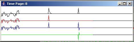 |
Figure 8 |
Interpretation of the traces
Regardless of whether the user has opted for an identification filter or an inverse filter, the four traces shown in Figure 8 have the same relationship to the adaptive engine.
However, depending on whether the user has opted for an identification filter or an inverse filter, the specific time series that are fed to the adaptive engine for the first two roles in the above list are different.
For an identification filter, the wideband test data is fed to the adaptive engine as the input to the adaptive filter and the path output data is fed to the adaptive engine as the target. See the picture at The MathWorks web site.
For an inverse filter, the path output data is fed to the adaptive engine as the input to the adaptive filter, and the wideband data is fed to the adaptive engine as the target. See the other picture at The MathWorks web site.
The top two traces are switched
In summary, the top two traces in graphs having the format of Figure 8 are switched depending on whether the user has opted for an identification filter or an inverse filter.
The data traces for Figure 8
Because Figure 8 shows the time series involved in the development of an inverse filter, the black top trace in Figure 8 is the path output data. The wideband test data is shown by the red trace. As always, the adaptive filter output is shown by the blue trace, and the error is shown by the green trace.
The top panel in Figure 8 shows these traces at the beginning of the run and the bottom panel shows these traces at the end of the run.
As you can see in the bottom panel of Figure 8, the blue filter output trace matches the red target trace. The green error trace, which is the difference between the adaptive filter output and the target, has been driven to zero.
Impulse responses
The bottom panel in Figure 8 shows two sets of impulses or wavelets, one following the other in time. The left-most set of wavelets in Figure 8 has the same meaning as in Figure 5, except for the reversal of the top two traces. In this case, the impulse that is inserted in the wideband data is shown in the red trace. The impulse response of the path is shown in the black trace, and it matches the impulse response shown in Figure 4 as before.
Now for something a little different
The leftmost wavelet on the blue trace in Figure 8 shows the result of applying the adaptive filter, which is now an inverse filter instead of an identification filter to the path output data. In this case, the inverse filter has acted on the wavelet shown in the black path output trace and has transformed it back into a single impulse that matches the impulse in the wideband test data shown by the red trace. That is the desired result. The inverse filter has compensated for, or cancelled out, the characteristics of the path, producing an output that matches the input to the path.
The rightmost wavelets
Now consider the rightmost set of wavelets in the bottom panel in Figure 8. At the time of the rightmost set of wavelets, an impulse was inserted into the black path output data. This impulse propagated through the adaptive filter, (for which the state had been frozen by disabling adaptive updates) producing the impulse response of the adaptive filter shown by the rightmost wavelet on the blue trace.
What does this all mean?
One way to think of this is as follows. The red impulse in the wideband test data was convolved with the impulse response of the path producing the output shown by the leftmost black wavelet. This wavelet was convolved with the impulse response of the adaptive filter (shown by the rightmost blue wavelet) producing the leftmost blue wavelet. For an inverse filter, the leftmost blue wavelet is an impulse that matches (or tries to match) the original input to the path shown by the red trace.
(The wavelet on the green error trace in Figure 8 is an artifact that has no meaning in this discussion of impulse responses. Just ignore it.)
The impulse and frequency response of the adaptive filter
Now let's take a look at the impulse and frequency response of the adaptive filter as shown in Figure 9.
The impulse response of the adaptive filter is shown in the left panel of Figure 9, progressing from the beginning to the end of the run. You should recognize the impulse response at the bottom of the left panel in Figure 9 as the same impulse response that you saw as the rightmost blue wavelet in Figure 8.
 |
 |
Figure 9 |
|
The frequency response of the adaptive filter
The amplitude and phase response of the adaptive filter is shown in the right panel of Figure 9 with time progressing down the page. As before, the phase response (shown in red) is flat. This makes us happy.
Note the shape of the black amplitude response at the bottom of the right panel. Compare it with the amplitude response of the path shown in Figure 4. As you can see, the amplitude response of the adaptive filter is the inverse of the amplitude response of the path.
At low frequencies where the amplitude response of the path is high, the amplitude response of the inverse adaptive filter is low. At high frequencies where the amplitude response of the path is low, the amplitude response of the inverse filter is high. The result is that the product of these two frequency responses (on a frequency by frequency basis) produces an overall response that is very flat across the frequency spectrum from zero to the Nyquist folding frequency.
More evidence
This is borne out by the graph shown in Figure 10. Figure 10 shows the amplitude and phase response of a wavelet produced by convolving the impulse response of the path with the impulse response of the inverse filter.
Figure 10 |
Essentially, Figure 10 shows the amplitude and phase response of a wavelet that matches the leftmost blue wavelet in Figure 8. Because this wavelet is an impulse, the amplitude response is flat across all frequencies and the phase response is zero across all frequencies.
We already knew that the amplitude response of an impulse was flat
I'm showing you the graph in Figure 10 at this point in the discussion mainly to prepare you for corresponding graphs for other path scenarios. As you will see later, some of the corresponding graphs for other path scenarios aren't nearly as ideal as this one.
Where do we go from here?
I don't plan to show you nearly this much detail for all six path scenarios that are built into the program. You can run all of the scenarios and view the details for yourself. However, I will show you the highlights for a couple of additional path scenarios.
A path with multiple echoes
At this point, I am going to skip ahead to the path scenario identified as test case number 5. The parameters for this run are shown in Figure 11. As you can see from Figure 11, this run is intended to develop an identification filter.
Input values were provided.
Using following values:
feedbackGain: 1.0E-4
numberIterations: 2001
filterLength: 26
testCase: 5
identification: true
Figure 11 |
The path characteristics
Let's begin with the path characteristics shown in Figure 12.
 |
 |
Figure 12 |
|
The impulse response of the path is shown in the left panel of Figure 12. The amplitude and phase response of the path is shown in the right panel of Figure 12.
Multiple echoes
If by now you have developed an understanding of the convolution process, you may recognize that the impulse response shown in Figure 12 causes the path output to consist of the sum of four attenuated versions of the input, each delayed relative to the previous one. This is generally what we would hear in an acoustic echo situation.
Hello
Hello
Hello
Hello
The amplitude response
This results in a path amplitude response that is definitely not flat as shown by the right panel of Figure 12. In fact, this results in a situation where destructive interference causes (almost) total suppression of the signal at one frequency.
(Note that the phase also goes through a little nonlinearity at the frequency where the amplitude response goes to near zero.)
The adaptive time series
Figure 13 shows the beginning and the ending time series for this run. As you can see, by the end of the run, the green error has been driven to zero and the impulse response of the adaptive filter shown by the blue wavelet matches the impulse response of the path shown in red. Thus, the unknown characteristics of the path have been faithfully captured in the adaptive filter. (The unknown characteristics of the path have been identified.)
 |
 |
Figure 13 |
If you run this case and view the amplitude and phase response for the adaptive filter, you will see that they are also a good match for the amplitude and phase response for the path shown in Figure 12.
Inverse filter for path with multiple echoes
Now let's develop the inverse filter for the same path with multiple echoes. The input parameters for this case are shown in Figure 14.
Input values were provided.
Using following values:
feedbackGain: 1.0E-4
numberIterations: 2001
filterLength: 26
testCase: 5
identification: false
Figure 14 |
The time series for the inverse adaptive filter
The beginning and ending time series for the run are shown in Figure 15.
 |
 |
Figure 15 |
This is a little different
Note that in Figure 15, unlike for the previous path scenario, the green error trace was not driven completely to zero.
Perhaps the most striking thing about Figure 15 is that the impulse response of the adaptive filter (shown as the rightmost blue wavelet) did not succeed in fully compensating for the path characteristics. This is evidenced by the fact that the leftmost blue wavelet is not a clean impulse. Rather, there is some noise to the right of the main body of that wavelet.
How do we explain this anomaly?
I will begin the explanation by taking a look at the impulse and frequency response of the adaptive filter shown in Figure 16 and comparing it with the frequency response of the path shown earlier in Figure 12.
 |
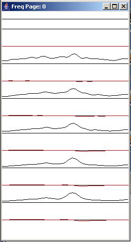 |
Figure 16 |
|
Reality sets in
The reality is that it is not possible to develop a perfect inverse filter for this path. There is a frequency (see Figure 12) at which the frequency response of the path totally suppresses (or at least almost totally suppresses) the energy propagating through the path. Once that energy is gone, there is nothing that an inverse filter can do to recover it.
A peak in the amplitude response
If you look at the bottom amplitude response shown in Figure 16, there is a peak in the amplitude response at that frequency. However, for that peak to function as the inverse of the notch in the frequency response of the path (see Figure 12) at that frequency, the peak would have to be infinite in height (or at least very large), which it clearly isn't.
Very little energy in the output at that frequency
Continuing with the explanation as to why the inverse filter doesn't totally compensate for the path characteristics, Figure 17 shows the amplitude and phase response for the wavelet produced by convolving the impulse response of the path with the impulse response of the adaptive filter (the leftmost blue wavelet in Figure 15).
Figure 17 |
Unlike the previous case shown in Figure 10, this amplitude response is not completely flat. Rather, it has a notch at the frequency where the amplitude response of the path goes through zero.
Again, once the characteristics of the path have suppressed most of the energy at that frequency, there is nothing that the inverse filter can do to recreate that energy.
A path with four notches
If you run case 6, you will see that it exhibits similar behavior but even worse. I purposely designed this case such that the amplitude response of the path has four points where the amplitude response goes through zero, as shown in Figure 18.
Figure 18 |
The output time series
This results in the time series shown in Figure 19. As you can see, the adaptive inverse filter (the rightmost blue wavelet in Figure 19) does not succeed in totally compensating for the path characteristics. There is quite a bit of noise following the main body of the leftmost blue wavelet in Figure 19.
Figure 19 |
Also, the green error trace has not been driven to zero in Figure 19.
The overall frequency response
The amplitude and phase spectrum of the leftmost blue wavelet in Figure 19 is shown in Figure 20. As you can see, there are four notches in the spectrum at the same frequencies as the points where the amplitude response of the path (shown in Figure 18) goes through zero. Also, there are nonlinearities in the phase response at those frequencies.
Figure 20 |
The input parameters
For the record, the input parameters for this run are shown in Figure 21.
Input values were provided.
Using following values:
feedbackGain: 1.0E-4
numberIterations: 2001
filterLength: 26
testCase: 6
identification: false
Figure 21 |
Brief summary of adaptive inverse filtering
In summary, inverse filtering can do a lot to compensate for path characters and to restore a signal to the form that it had before propagating through the path. Inverse filtering can amplify energy that has been attenuated by the path, and can often correct for phase distortion. However, inverse filtering cannot work miracles. It cannot recreate signal energy that has been totally eliminated by the path. Fortunately most real-world paths are probably closer to the situation illustrated by case number 1 than by cases 5 and 6.
Now let's see some code.
The class named Adapt07
Listing 1 contains the beginning of the class named Adapt07 and the entire main method.
class Adapt07{
  public static void main(String[] args){
    //Default parameter values
    double feedbackGain = 0.0001;
    int numberIterations = 2001;
    int filterLength = 26;//Must be >= 26 for plotting.
    //Six test cases, numbered 1 through 6 are defined
    // later.
    int testCase = 1;
    //A value of true for the following variable causes the
    // adaptive process to attempt to develop an
    // identification filter. A value of false causes the
    // adaptive process to attempt to develop an inverse
    // filter for the path impulse response.
    boolean identification = true;

    //The following scale factor is applied to the
    // wideband test data.  This is not an input
    // parameter.
    double wbTestDataScale = 10;

    //Process command-line arguments.  Note that because of
    // plotting alignment issues discussed in earlier
    // lessons, the filter length must be at least 26.
    if(args.length != 5){
      System.out.println(
               "Usage with all parameters following the " +
               "program name:\n" +
               "java Adapt07\n" +
               "feedbackGain\n" +
               "numberIterations\n" +
               "filterLength >= 26\n" +
               "testCase, 1 to 9\n" +
               "identification, T or F\n");

      System.out.println(
          "Input values were not provided.\n"+
          "Using following default values:\n" +
          "feedbackGain: " + feedbackGain +
          "\nnumberIterations: " + numberIterations +
          "\nfilterLength: " + filterLength +
          "\ntestCase: " + testCase +
          "\nidentification: " + identification);
    }else{//Command line params were provided.
      feedbackGain = Double.parseDouble(args[0]);
      numberIterations = Integer.parseInt(args[1]);
      filterLength = Integer.parseInt(args[2]);
      //FilterLength must be 26 or greater to avoid
      // plotting alignment problems.
      if(filterLength < 26){
        System.out.println(
                   "\nfilterLength must be 26 or greater");
        System.out.println("Termnating program");
        System.exit(0);
      }//end if
      testCase = Integer.parseInt(args[3]);
      if(args[4].toUpperCase().equals("T")){
        identification = true;
      }else{
        identification = false;
      }//end else

      System.out.println(
          "Input values were provided.\n"+
          "Using following values:\n" +
          "feedbackGain: " + feedbackGain +
          "\nnumberIterations: " + numberIterations +
          "\nfilterLength: " + filterLength +
          "\ntestCase: " + testCase +
          "\nidentification: " + identification);
    }//end else

    //Instantiate a new object of the Adapt07 class
    // and invoke the method named process on that object.
    new Adapt07().process(feedbackGain,
                          numberIterations,
                          filterLength,
                          wbTestDataScale,
                          testCase,
                          identification);
  }//end main

Listing 1
|
The code in Listing 1 is completely straightforward and shouldn't require any explanation beyond the comments contained in the code.
Note that the main method instantiates an object of the Adapt07 class and invokes the instance method named process on that object.
The process method
Listing 2 shows the beginning of the method named process.
  void process(double feedbackGain,
               int numberIterations,
               int filterLength,
               double wbTestDataScale,
               int testCase,
               boolean identification){

    //The following array will be populated with the
    // adaptive filter for display purposes.
    double[] filter = null;

Listing 2
|
The code in Listing 2 is also completely straightforward.
Six built in path scenarios
Things begin to get interesting in Listing 3. The code in Listing 3 instantiates and initializes six array objects to contain the coefficient values for the six path scenarios described earlier. Each array object contains the coefficient values for the impulse response of a particular path scenario.
    //Define several test cases for the path impulse
    // response.

    //Low-pass filter with short time constant.
    double[] pathA = {1.0,
                      0.5,
                      0.25,
                      0.125,
                      0.0625,
                      0.03125,
                      0.015625,
                      0.0};

    //Low-pass filter with long time constant.
    double[] pathB = {1.0,
                      0.8,
                      0.64,
                      0.512,
                      0.4096,
                      0.32768,
                      0.262144,
                      0.2097152,
                      0.1677721,
                      0.1342176,
                      0.1073740,
                      0.0858992,
                      0.0687193,
                      0.0549754,
                      0.0439803,
                      0.0351842,
                      0.0};

    //High-pass filter with long time constant.
    double[] pathC = {1.0,
                     -0.8,
                      0.64,
                     -0.512,
                      0.4096,
                     -0.32768,
                      0.262144,
                     -0.2097152,
                      0.1677721,
                     -0.1342176,
                      0.1073740,
                     -0.0858992,
                      0.0687193,
                     -0.0549754,
                      0.0439803,
                     -0.0351842,
                      0.0};

    //Mid-pass filter with long time constant.
    double[] pathD = {1.0,
                      0.0,
                     -0.64,
                      0.0,
                      0.4096,
                      0.0,
                     -0.262144,
                      0.0,
                      0.1677721,
                      0.0,
                     -0.1073740,
                      0.0,
                      0.0687193,
                      0.0,
                     -0.0439803,
                      0.0};

    //Simulation of an acoustic signal with echoes.
    double[] pathE = {1.0,
                      0.0,
                      0.64,
                      0.0,
                      0.0,
                      0.32768,
                      0.0,
                      0.0,
                      0.0,
                      0.1342176,
                      0.0,
                      0.0,
                      0.0,
                      0.0,
                      0.0439803,
                      0.0};

    //Digital boxcar filter with peak at half the folding
    // frequency.
    double[] pathF = {1.0,
                      0.0,
                     -1.0,
                      0.0,
                      1.0,
                      0.0,
                     -1.0};

Listing 3
|
Selection of a path scenario
The code in Listing 4 uses the command-line parameter named testCase to select one of the six path scenarios for the run. This code is straightforward.
    //A reference to the selected path operator will be
    // stored here.
    double[] pathOperator = null;

    if(testCase == 1){
      pathOperator = pathA;
    }else if(testCase == 2){
      pathOperator = pathB;
    }else if(testCase == 3){
      pathOperator = pathC;
    }else if(testCase == 4){
      pathOperator = pathD;
    }else if(testCase == 5){
      pathOperator = pathE;
    }else if(testCase == 6){
      pathOperator = pathF;
    }else{
      System.out.println("Invalid testCase");
      System.out.println("Terminating program");
      System.exit(0);
    }//end else

Listing 4
|
You are encouraged to experiment
Three of the path scenarios defined in Listing 3 and selected in Listing 4 were described or partially described in the earlier section titled Experimental Results. You are encouraged to run the program for all six of the scenarios (by specifying the appropriate command-line parameters) and to examine the results. See if you can explain the results for each of the six scenarios.
You are also encouraged to modify the coefficient values in one or more of the array objects in Listing 3 to create your own path scenarios. Then recompile and run the program for your scenarios. See if you can explain the results.
See if you can create path scenarios for which either the identification filter or the inverse filter fails to converge to a solution. If so, see if you can explain why the LMS adaptive algorithm won't converge for that path scenario.
Display the pathOperator and its frequency response
The code in Listing 5 uses capabilities previously described in earlier lessons referred to in the References section to display the impulse response and the frequency response of the path as shown in Figure 4 and Figure 12.
    //Display the pathOperator
    //First instantiate a plotting object.
    PlotALot01 pathOperatorObj = new PlotALot01("Path",
               (pathOperator.length * 4) + 8,148,70,4,0,0);

    //Feed the data to the plotting object.
    for(int cnt = 0;cnt < pathOperator.length;cnt++){
      pathOperatorObj.feedData(40*pathOperator[cnt]);
    }//end for loop

    //Cause the graph to be displayed on the computer
    // screen in the upper left corner.
    pathOperatorObj.plotData(0,0);

    //Now compute and plot the frequency response of the
    // selected path

    //Instantiate a plotting object for two channels of
    // frequency response data.  One channel is for
    // the amplitude and the other channel is the phase.
    PlotALot03 pathFreqPlotObj =
                   new PlotALot03("Path",264,148,35,2,0,0);

    //Compute the frequency response and feed the results
    // to the plotting object.
    displayFreqResponse(pathOperator,pathFreqPlotObj,
                                                    128,0);

    //Cause the frequency response data stored in the
    // plotting object to be displayed on the screen in
    // the top row of images.
    pathFreqPlotObj.plotData(112,0);

Listing 5
|
If you have been studying the code in the earlier lessons in this series (see References) the code in Listing 5 should not require further explanation.
Instantiate an adaptive engine object
Listing 6 instantiates an object of the AdaptEngine02 class to handle the adaptive behavior of the program. The use of the class named AdaptEngine02 is new to this lesson. You can view a complete listing of the class named AdaptEngine02 in Listing 18 near the end of the lesson.
    AdaptEngine02 adapter = new AdaptEngine02(
                                filterLength,feedbackGain);

Listing 6
|
Although the class named AdaptEngine02 is new to this lesson, it is very similar to the class named AdaptEngine01 that has been used and explained in several of the earlier lessons referred to in the References section. The only thing new in the AdaptEngine02 class is the ability to temporarily enable or disable the updating of the adaptive filter coefficients for each adaptive iteration by passing a boolean parameter to the adapt method. Therefore, I won't provide a further explanation of the AdaptEngine02 class in this lesson.
Declare working objects and variables
Listing 7 declares and initializes some working objects and working variables that will be used later in the program. This code is straightforward and should not require further explanation
    //Instantiate an array object that will be used as a
    // delay line for the wideband test data.
    double[] rawData = new double[pathOperator.length];

    //Instantiate a plotting object for four channels of
    // time-serie data.
    PlotALot05 timePlotObj =
                   new PlotALot05("Time",468,148,25,2,0,0);

    //Instantiate a plotting object for two channels of
    // filter frequency response data.  One channel is for
    // the amplitude and the other channel is for the
    // phase.
    PlotALot03 freqPlotObj =
                   new PlotALot03("Freq",264,487,35,2,0,0);

    //Instantiate a plotting object to display the filter
    // impulse response at specific time intervals during
    // the adaptive process.
    PlotALot01 filterPlotObj = new PlotALot01("Filter",
                     (filterLength * 4) + 8,487,70,4,0,0);

    //Declare and initialize working variables.
    double output = 0;
    double err = 0;
    double target = 0;
    double input = 0;
    double wbTestData = 0;
    boolean adaptOn;

Listing 7
|
Execute adaptive iterations
Listing 8 shows the beginning of a for loop that causes the program to execute the specified number of adaptive iterations.
    for(int cnt = 0;cnt < numberIterations;cnt++){

      adaptOn = true;

Listing 8
|
Enabling and disabling adaptive coefficient updates
The variable named adaptOn, which is set to true in Listing 8, is used to enable and disable the adaptive filter coefficient update process in the adapt method of the adaptive engine. As you will see later, this variable is passed as the third parameter to the adapt method.
When the value of that parameter is true, the adapt method uses the adaptive error to update the coefficient values in the adaptive filter. When that parameter is false, the coefficient values are not updated during that call to the adapt method.
Adaptive updates are disabled near the end of the run
The value of adaptOn is allowed to remain true during most of the adaptive iterations in this program. However, near the end of the run, this value is set to false to disable the adaptive update and to freeze the adaptive filter in its current state. Then two different impulses are inserted into the test data to produce the impulse responses shown in Figure 5, Figure 8, Figure 13, Figure 15, and Figure 19.
As with the use of the class named AdaptEngine02, this feature is new to this program, and I will explain how it is accomplished in more detail later.
Get wideband test data
Listing 9 gets and scales the next sample of wideband test data from a random number generator. Before scaling by wbTestDataScale, the values are uniformly distributed from -1.0 to 1.0.
      wbTestData =
                 wbTestDataScale*(2*(Math.random() - 0.5));

Listing 9
|
Insert an impulse in the wideband test data
Listing 10 sets the wideband input values near the end of the run to zero and turns adaptation off by setting the value of adaptOn to false. Listing 10 also inserts an impulse into the wideband test data near the end of the run.
That impulse, which is shown on the red trace in the leftmost set of wavelets in Figure 19, produces the leftmost wavelets that appear in the other traces in Figure 19. Among other things, this causes the impulse response of the path to be visible as the leftmost wavelet in the black trace in Figure 19.
      //Set wideband test data to zero
      if(cnt > (numberIterations - 5*filterLength)){
        wbTestData = 0;
        adaptOn = false;
      }//end if

      //Now insert an impulse at one specific location in
      // the wideband test data.
      if(cnt == numberIterations - 3*filterLength){
        wbTestData = 2 * wbTestDataScale;
      }//end if

Listing 10
|
Apply the path operator to the wideband test data
Listing 11 inserts the wideband test data into the rawData delay line and then invokes the reverseDotProduct method to perform one step in the convolution of the raw data with the path operator.
      //Insert the wideband test data into the raw data
      // delay line.
      flowLine(rawData,wbTestData);

      //Apply the path operator to the wideband test data.
      // Note the use of the method named
      // reverseDotProduct, which is new to this lesson.
      // This method provides the time reversal that is
      // necessary for true convolution.
      double pathData =
                   reverseDotProduct(rawData,pathOperator);

Listing 11
|
The method named reverseDotProduct
Note that the method named reverseDotProduct is new to this lesson. (You can view the lesson in its entirety in Listing 17.) However, it is very similar to the method named dotProduct, which has been used in various previous lessons referred to in the section titled References. The only significant difference between this new version of the method named reverseDotProduct and the earlier version named dotProduct is that this new version reverses the time order of the operator coefficients before computing the vector dot product. This is consistent with the requirement to reverse the time order of the operator coefficients before performing a convolution operation.
Because of the similarity of the new version of the method with the version that was used and explained in earlier lessons, I won't discuss the method named reverseDotProduct further in this lesson.
Declare another working variable
Listing 12 declares a variable of the AdaptiveResult class, which will receive a reference from the adapt method containing various results of the adaptive process.
AdaptiveResult result = null; Listing 12 |
Develop an identification filter
Listing 13 shows the beginning of an if statement that:
      if(identification){//Develop an identification filter
        //Establish input values.
        input = wbTestData;
        target = pathData;
        //Do the adaptive processing.
        result = adapter.adapt(input,target,adaptOn);

Listing 13
|
Develop an inverse filter
Listing 14 shows the else clause of the if statement that began in Listing 13. The else clause:
      }else{//Develop an inverse filter.
        //Establish input values.
        input = pathData;
        target = wbTestData;

        //Insert an impulse into the pathData.
        if(cnt == numberIterations - filterLength){
          input = 2 * wbTestDataScale;
        }//end if

        //Do the adaptive processing
        result = adapter.adapt(input,target,adaptOn);
      }//end else

Listing 14
|
Inserting the impulse
When the run is nearly complete adaptive updates are disabled and the wideband input data values are set to zero by the code in Listing 10. That code also inserts an impulse in the wideband test data.
Listing 14 inserts an impulse into the path output data values. (This happens later than the point in time where the impulse was inserted into the wideband test data by the code in Listing 10.) This impulse is shown in the black trace in the rightmost set of wavelets in Figure 19. The existence of the impulse in the input to the adaptive filter causes the impulse response of the adaptive filter to be displayed as the rightmost wavelet in the blue trace in Figure 19.
Plot adaptive results, etc.
The code in Listing 15:
      //Get and save adaptive results for plotting and
      // spectral analysis
      output = result.output;
      err = result.err;
      filter = result.filterArray;

      //Feed the time series data to the plotting object.
      timePlotObj.feedData(input,target,output,-err);

      //Compute and plot summary results at the end of
      // every 400th iteration.
      if(cnt%400 == 0){
        displayFreqResponse(filter,freqPlotObj,
                                    128,filter.length - 1);

        //Display the filter impulse response coefficient
        // values.  The adaptive engine returns the filter
        // with the time axis reversed relative to the
        // conventional display of an impulse response.
        // Therefore, it is necessary to display it in
        // reverse order.
        for(int ctr = 0;ctr < filter.length;ctr++){
          filterPlotObj.feedData(
                       40*filter[filter.length - 1 - ctr]);
        }//end for loop
      }//End display of frequency response and filter
    }//End for loop,

    //Cause the data stored in the plotting objects to be
    // plotted.
    timePlotObj.plotData(376,0);//Top of screen
    freqPlotObj.plotData(0,148);//Left side of screen
    filterPlotObj.plotData(265,148);

Listing 15
|
If you have been studying the earlier lessons in this series referred to in the References section, you will find the code in Listing 15 to be very familiar and straightforward.
Convolve adaptive filter with the path operator
For the case of an inverse filter only, the code in Listing 16 convolves the adaptive filter with the impulse response of the path to determine the extent to which the filter is able to compensate for the characteristics of the path.
This determination is made by computing the amplitude and phase spectrum of the wavelet that is produced by the convolution, and displaying that frequency-domain information in the format shown in Figure 20. If the filter is a true inverse filter for the path, the amplitude spectrum will be flat and the phase will be either zero or linear (indicating a time delay). Deviations such as those shown in Figure 20 indicate that the inverse filter has some shortcomings.
    if(!identification){
      //Copy the filter into another array with zeros on
      // both ends to account for end effects in the
      // convolution process.
      double[] convInput = new double[
                    filter.length + 2*pathOperator.length];
      for(int cnt = 0;cnt < filter.length;cnt++){
        convInput[cnt + pathOperator.length] = filter[cnt];
      }//end for loop

      //Create an array to receive the convolution output.
      double[] convOutput =
           new double[filter.length + pathOperator.length];

      //Call the method named convolve01 to perform the
      // convolution.
      convolve01(convInput,pathOperator,convOutput);

      //Now compute and plot the frequency spectrum of the
      // time series that results from convolving the final
      // adaptive filter with the path impulse response.
      // Ideally, the amplitude response will be flat from
      // zero to the folding frequency and the phase
      // response will be flat, or possibly linear
      // (indicating a time delay).

      //Instantiate a plotting object for two channels of
      // frequency response data.  One channel is for
      // the amplitude and the other channel is the phase.
      PlotALot03 finalFreqPlotObj =
                  new PlotALot03("Final",264,137,35,2,0,0);

      //Compute the frequency response and feed the results
      // to the plotting object.
      displayFreqResponse(convOutput,finalFreqPlotObj,
                                128,convOutput.length - 1);

      //Cause the frequency response data stored in the
      // plotting object to be displayed on the screen.
      finalFreqPlotObj.plotData(
                           265 + filterLength * 4 + 8,148);
    }//end if

  }//end process method

Listing 16
|
Although the code in Listing 16 is rather long, with one exception it is straightforward and uses capabilities explained in earlier lessons in this series. (See the section titled References.) Therefore, I won't explain the code in Listing 16 further in this lesson.
The convolve01 method
The one exception has to do with the use of the method named convolve01. This method is very similar to a method that I presented and explained in an earlier lesson titled Convolution and Frequency Filtering in Java, so I won't repeat that explanation here. You can view the code for the method named convolve01 in Listing 17 near the end of the lesson.
I encourage you to copy the code from the classes in the section titled Complete Program Listings. Compile and execute the programs. Experiment with the code. Make changes to the code, recompile, execute, and observe the results of your changes.
Run all six of the built-in cases and see if you can explain the results.
After running the built-in cases, you might want to modify the filter coefficients for one of the path operators shown in Listing 3. Then recompile and run the program and observe the results. Did your change cause the results to be different? If so, how were they different? See if you can explain why they were different.
You might also try to come up with a set of path coefficients for which the adaptive process fails to converge, both for an identification filter and for an inverse filter. If your changes cause either or both processes to fail to converge, see if you can explain the reasons why?
While you are at it, experiment with different values for feedBackGain. What happens if you use a large value for feedbackGain? What happens if you use a very small value for feedbackGain? What happens if you use a negative value for feedbackGain? Can you explain the results that you experience?
While experimenting with the feedbackGain, you might also want to experiment with the command-line parameter named numberIterations. See if you can explain the results for small, medium, and large values for this parameter.
Other classes required
In addition to the classes named Adapt07, AdaptEngine02, and AdaptiveResult (for which the source code is provided in this lesson), you will need access to the following classes. The source code for these classes can be found in the lessons indicated.
In this lesson, I showed you how to use a general-purpose LMS adaptive engine to write a Java program that illustrates adaptive identification filtering and adaptive inverse filtering for different path scenarios.
Adaptive filtering is commonly used for the following four scenarios:
This lesson explains how to write Java programs to work in the first two scenarios in the list. I plan to publish lessons that explain and provide examples of the remaining two scenarios in future lessons.
In preparation for understanding the material in this lesson, I recommend that you study the material in the following previously-published lessons:
Links to the lessons in the above list are available at Digital Signal Processing-DSP.
Complete listings of the classes discussed in this lesson are shown in the listings below.
/*File Adapt07.java.java
Copyright 2005, R.G.Baldwin

The purpose of this program is to illustrate adaptive
identification and inverse identification.

Further information on these two topics can be found at the
following three web sites:

www.eee.strath.ac.uk/r.w.stewart/adaptivejava/begin.htm

www.mathworks.com/access/helpdesk/help/toolbox/
filterdesign/adaptiv5.html#5547

www.mathworks.com/access/helpdesk/help/toolbox/
filterdesign/adaptiv6.html#5557

This program requires the following classes:
Adapt07.class
AdaptEngine02.class (new to this lesson)
AdaptiveResult.class
ForwardRealToComplex01.class
PlotALot01.class
PlotALot03.class
PlotALot05.class

This program uses the adaptive engine named AdaptEngine02
to adaptively develop a filter.  Depending on user input,
the filter is either an identification filter or an inverse
filter.

The class named AdaptEngine02 is an upgrade to the class
named AdaptEngine01 that was used in earlier programs.
This upgrade makes it possible for the user to pass a
boolean parameter to the adapt method of the engine to
either enable or disable the adaptive update of the filter
coefficients.

When the filter is an identification filter, the adaptive
process attempts to replicate the impulse response of a
path through which wideband test data are flowing.

When the filter is an inverse filter, the adaptive process
attempts to develop a filter that is the inverse of the
impulse response of a path through which wideband test
data are flowing.

User-selectable test cases are provided for six different
path scenarios. The user may develop an identification
filter or an inverse filter for any of the six cases.

If the user opts for an identification filter, five
separate graphs are produced. If the user opts for an
inverse filter, six separate graphs are produced.  The
graphs appear on the screen in two rows with three graphs
in each row.

The following is a brief description of each of the six
graphs, working from left to right across the top row and
then working from left to right across the second row.

1.  The impulse response of the path through which the wide
band data are flowing.
2.  The amplitude and phase response of the path through
which the wideband data are flowing.
3.  Four time series that illustrate the time behavior of
the adaptive process.  The adaptive behavior is disabled
and impulses are appended onto the ends of the input time
series to cause the impulse response of various filters to
be displayed at the ends of the time series in this graph.
4.  The amplitude and phase response of the adaptive filter
at the end of every 400th iteration.
5.  The impulse response of the adaptive filter at the end
of every 400th adaptive iteration.
6.  The amplitude and phase spectrum of the time series
produced by convolving the final adaptive filter with the
impulse response of the path.  This graph is produced only
when the filter being developed is an inverse filter.  This
amplitude and phase spectrum illustrates the extent to
which the inverse filter is able to compensate for the path
characteristics.  Ideally the amplitude spectrum is flat
and the phase spectrum is either flat or linear
(indicating a time delay).

Graphs 3, 4, and 5 consist of multiple pages stacked on top
of one another.  Move the pages on the top of the stack to
view the pages further down.  The pages on the top of the
stack represent the results produced early in the adaptive
process while those further down represent the results
produced later in the adaptive process.

The four time series that are plotted are, from top to
bottom in the colors indicated:
1.  Input to the adaptive filter (black).
2.  Target for the adaptive process (red).
3.  Output from the adaptive filter (blue).
4.  Error computed within the adaptive process (green).

Near the end of the run, the adaptive update process is
disabled.  The input data is set to zero for the remainder
of the run except that on two subsequent occasions, an
impulse is inserted into the data.  By running the same
path twice, once in identification mode and once in inverse
filter mode, this makes it possible to see:

1. The impulse response of the path.
2. The impulse response of the final adaptive
identification filter.
3. The extent to which the impulse response of the
identification filter matches the impulse response of the
path.
4. The impulse response of the final inverse filter.
5  The extent to which the convolution of the inverse
filter with the impulse response of the path compensates
for the characteristics of the path and produces the ideal
output consisting of a single impulse.

In operation, the program generates wideband test data
produced by a random number generator and convolves it with
a specified path impulse response to simulate the impact of
the path on the wideband test data.  The original
wideband test data and the path output data are both
presented to the adaptive engine.

When the original wideband test data is presented as the
data to be filtered within the adaptive engine and the
path output is presented as the target, the adaptive
process attempts to develop an adaptive filter that
replicates the impulse response of the path.

When the two are reversed, the adaptive process attempts to
develop an adaptive filter that is the inverse of the
impulse response of the path.

User input is provided by five command-line parameters.  If
no command-line parameters are provided, default parameters
are used.

The command-line parameters are:

feedbackGain: The gain factor that is used in the feedback
loop to adjust the coefficient values in the adaptive
filter.

numberIterations: This is the number of iterations that the
program executes before stopping and displaying all of the
graphic results.

filterLength: This is the number of coefficients in the
adaptive filter.  Must be at least 26.

testCase:  An integer from 1 to 9 that specifies the
simulated path scenario.

identification:  Input is T or F.  T specifies that the
adaptive process is to develop an identification filter.
F specifies that the adaptive process is to develop an
inverse filter.

The minimum filter length of 26 has to do with plotting
alignment issues and has nothing to do with the adaptive
process.  See a description of the alignment issues in
earlier lessons.

The six path scenarios can be generally described as
follows:

1.  A low-pass filter of the sort that might be realized
with a passive RC network.
2,  Another low-pass filter that might be realized with a
passive RC network but with a much longer time constant
than scenario 1.
3.  A high-pass filter of the sort that might be realized
with a passive RLC network having the same long time
constant as scenario 2.
4,  A mid-band filter of the sort that might be realized
with a passive RLC network having the same long time
constant as scenarios 2 and 3.
5.  A filter that might represent an acoustic signal in
the presence of echoes.
6.  A boxcar digital filter with a peak at half the
Nyquist folding frequency.

Tested using J2SE 5.0 and WinXP.  J2SE 5.0 or later is
required.
**********************************************************/
import static java.lang.Math.*;//J2SE 5.0 req

class Adapt07{
  public static void main(String[] args){
    //Default parameter values
    double feedbackGain = 0.0001;
    int numberIterations = 2001;
    int filterLength = 26;//Must be >= 26 for plotting.
    //Six test cases, numbered 1 through 6 are defined
    // later.
    int testCase = 1;
    //A value of true for the following variable causes the
    // adaptive process to attempt to develop an
    // identification filter. A value of false causes the
    // adaptive process to attempt to develop an inverse
    // filter for the path impulse response.
    boolean identification = true;

    //The following scale factor is applied to the
    // wideband test data.  This is not an input
    // parameter.
    double wbTestDataScale = 10;

    //Process command-line arguments.  Note that because of
    // plotting alignment issues discussed in earlier
    // lessons, the filter length must be at least 26.
    if(args.length != 5){
      System.out.println(
               "Usage with all parameters following the " +
               "program name:\n" +
               "java Adapt07\n" +
               "feedbackGain\n" +
               "numberIterations\n" +
               "filterLength >= 26\n" +
               "testCase, 1 to 9\n" +
               "identification, T or F\n");

      System.out.println(
          "Input values were not provided.\n"+
          "Using following default values:\n" +
          "feedbackGain: " + feedbackGain +
          "\nnumberIterations: " + numberIterations +
          "\nfilterLength: " + filterLength +
          "\ntestCase: " + testCase +
          "\nidentification: " + identification);
    }else{//Command line params were provided.
      feedbackGain = Double.parseDouble(args[0]);
      numberIterations = Integer.parseInt(args[1]);
      filterLength = Integer.parseInt(args[2]);
      //FilterLength must be 26 or greater to avoid
      // plotting alignment problems.
      if(filterLength < 26){
        System.out.println(
                   "\nfilterLength must be 26 or greater");
        System.out.println("Termnating program");
        System.exit(0);
      }//end if
      testCase = Integer.parseInt(args[3]);
      if(args[4].toUpperCase().equals("T")){
        identification = true;
      }else{
        identification = false;
      }//end else

      System.out.println(
          "Input values were provided.\n"+
          "Using following values:\n" +
          "feedbackGain: " + feedbackGain +
          "\nnumberIterations: " + numberIterations +
          "\nfilterLength: " + filterLength +
          "\ntestCase: " + testCase +
          "\nidentification: " + identification);
    }//end else

    //Instantiate a new object of the Adapt07 class
    // and invoke the method named process on that object.
    new Adapt07().process(feedbackGain,
                          numberIterations,
                          filterLength,
                          wbTestDataScale,
                          testCase,
                          identification);
  }//end main
  //-----------------------------------------------------//

  //This is the primary adaptive processing and plotting
  // method for the program.
  void process(double feedbackGain,
               int numberIterations,
               int filterLength,
               double wbTestDataScale,
               int testCase,
               boolean identification){

    //The following array will be populated with the
    // adaptive filter for display purposes.
    double[] filter = null;

    //Define several test cases for the path impulse
    // response.

    //Low-pass filter with short time constant.
    double[] pathA = {1.0,
                      0.5,
                      0.25,
                      0.125,
                      0.0625,
                      0.03125,
                      0.015625,
                      0.0};

    //Low-pass filter with long time constant.
    double[] pathB = {1.0,
                      0.8,
                      0.64,
                      0.512,
                      0.4096,
                      0.32768,
                      0.262144,
                      0.2097152,
                      0.1677721,
                      0.1342176,
                      0.1073740,
                      0.0858992,
                      0.0687193,
                      0.0549754,
                      0.0439803,
                      0.0351842,
                      0.0};

    //High-pass filter with long time constant.
    double[] pathC = {1.0,
                     -0.8,
                      0.64,
                     -0.512,
                      0.4096,
                     -0.32768,
                      0.262144,
                     -0.2097152,
                      0.1677721,
                     -0.1342176,
                      0.1073740,
                     -0.0858992,
                      0.0687193,
                     -0.0549754,
                      0.0439803,
                     -0.0351842,
                      0.0};

    //Mid-pass filter with long time constant.
    double[] pathD = {1.0,
                      0.0,
                     -0.64,
                      0.0,
                      0.4096,
                      0.0,
                     -0.262144,
                      0.0,
                      0.1677721,
                      0.0,
                     -0.1073740,
                      0.0,
                      0.0687193,
                      0.0,
                     -0.0439803,
                      0.0};

    //Simulation of an acoustic signal with echoes.
    double[] pathE = {1.0,
                      0.0,
                      0.64,
                      0.0,
                      0.0,
                      0.32768,
                      0.0,
                      0.0,
                      0.0,
                      0.1342176,
                      0.0,
                      0.0,
                      0.0,
                      0.0,
                      0.0439803,
                      0.0};

    //Digital boxcar filter with peak at half the folding
    // frequency.
    double[] pathF = {1.0,
                      0.0,
                     -1.0,
                      0.0,
                      1.0,
                      0.0,
                     -1.0};

    //A reference to the selected path operator will be
    // stored here.
    double[] pathOperator = null;

    if(testCase == 1){
      pathOperator = pathA;
    }else if(testCase == 2){
      pathOperator = pathB;
    }else if(testCase == 3){
      pathOperator = pathC;
    }else if(testCase == 4){
      pathOperator = pathD;
    }else if(testCase == 5){
      pathOperator = pathE;
    }else if(testCase == 6){
      pathOperator = pathF;
    }else{
      System.out.println("Invalid testCase");
      System.out.println("Terminating program");
      System.exit(0);
    }//end else

    //Display the pathOperator
    //First instantiate a plotting object.
    PlotALot01 pathOperatorObj = new PlotALot01("Path",
               (pathOperator.length * 4) + 8,148,70,4,0,0);

    //Feed the data to the plotting object.
    for(int cnt = 0;cnt < pathOperator.length;cnt++){
      pathOperatorObj.feedData(40*pathOperator[cnt]);
    }//end for loop

    //Cause the graph to be displayed on the computer
    // screen in the upper left corner.
    pathOperatorObj.plotData(0,0);

    //Now compute and plot the frequency response of the
    // selected path

    //Instantiate a plotting object for two channels of
    // frequency response data.  One channel is for
    // the amplitude and the other channel is the phase.
    PlotALot03 pathFreqPlotObj =
                   new PlotALot03("Path",264,148,35,2,0,0);

    //Compute the frequency response and feed the results
    // to the plotting object.
    displayFreqResponse(pathOperator,pathFreqPlotObj,
                                                    128,0);

    //Cause the frequency response data stored in the
    // plotting object to be displayed on the screen in
    // the top row of images.
    pathFreqPlotObj.plotData(112,0);

    //Instantiate an object to handle the adaptive behavior
    // of the program.  The use of the class named
    // AdaptEngine02 is new to this lesson.
    AdaptEngine02 adapter = new AdaptEngine02(
                                filterLength,feedbackGain);

    //Instantiate an array object that will be used as a
    // delay line for the wideband test data.
    double[] rawData = new double[pathOperator.length];

    //Instantiate a plotting object for four channels of
    // time-serie data.
    PlotALot05 timePlotObj =
                   new PlotALot05("Time",468,148,25,2,0,0);

    //Instantiate a plotting object for two channels of
    // filter frequency response data.  One channel is for
    // the amplitude and the other channel is for the
    // phase.
    PlotALot03 freqPlotObj =
                   new PlotALot03("Freq",264,487,35,2,0,0);

    //Instantiate a plotting object to display the filter
    // impulse response at specific time intervals during
    // the adaptive process.
    PlotALot01 filterPlotObj = new PlotALot01("Filter",
                     (filterLength * 4) + 8,487,70,4,0,0);

    //Declare and initialize working variables.
    double output = 0;
    double err = 0;
    double target = 0;
    double input = 0;
    double wbTestData = 0;
    boolean adaptOn;

    //Perform the specified number of iterations.
    for(int cnt = 0;cnt < numberIterations;cnt++){
      //The following variable is used to control whether
      // or not the adapt method of the adaptive engine
      // updates the filter coefficients when it is called.
      // The filters are updated when this variable is
      // true and are not updated when this variable is
      // false.
      adaptOn = true;

      //Get and scale the next sample of wideband test
      // data from a random number generator.  Before
      // scaling by wbTestDataScale, the values are
      // uniformly distributed from -1.0 to 1.0.
      wbTestData =
                 wbTestDataScale*(2*(Math.random() - 0.5));

      //Set wideband input values near the end of the run
      // to zero and turn adaptation off.  Insert an
      // impulse near the end that will produce several
      // interesting impulse responses.  Among other
      // things, this will cause the impulse response of
      // the path to be visible in the graphs.
      //Set values to zero.
      if(cnt > (numberIterations - 5*filterLength)){
        wbTestData = 0;
        adaptOn = false;
      }//end if
      //Now insert an impulse at one specific location in
      // the time series.
      if(cnt == numberIterations - 3*filterLength){
        wbTestData = 2 * wbTestDataScale;
      }//end if

      //Insert the wideband test data into the raw data
      // delay line.
      flowLine(rawData,wbTestData);

      //Apply the path operator to the wideband test data.
      // Note the use of the method named
      // reverseDotProduct, which is new to this lesson.
      // This method provides the time reversal that is
      // necessary for true convolution.
      double pathData =
                   reverseDotProduct(rawData,pathOperator);

      //Declare a variable that will be populated with the
      // results returned by the adapt method of the
      // adaptive engine.
      AdaptiveResult result = null;

      //Decide which type of filter to develop and do the
      // adaptive work.
      if(identification){//Develop an identification filter
        //Establish input values for the adaptive engine
        // that are appropriate for the development of
        // an identification filter.
        input = wbTestData;
        target = pathData;
        //Do the adaptive processing.
        result = adapter.adapt(input,target,adaptOn);
      }else{//Develop an inverse filter.
        //Establish input values for the adaptive engine
        // that are appropriate for the development of
        // an inverse filter.  Note that the input values
        // are reversed relative to an identification
        // filter.
        input = pathData;
        target = wbTestData;

        //When the run is nearly over and the wideband
        // input data values are zero, insert an impulse
        // into the pathData.  This happens later than the
        // point in time where the impulse was inserted
        // into the wideband test data. Note that
        // adaptation is still turned off at this point in
        // time.  Among other things, this makes it
        // possible to view the impulse response of the
        // inverse filter in the time series that are
        // displayed.
        if(cnt == numberIterations - filterLength){
          input = 2 * wbTestDataScale;
        }//end if

        //Do the adaptive processing
        result = adapter.adapt(input,target,adaptOn);
      }//end else

      //Get and save adaptive results for plotting and
      // spectral analysis
      output = result.output;
      err = result.err;
      filter = result.filterArray;

      //Feed the time series data to the plotting object.
      timePlotObj.feedData(input,target,output,-err);

      //Compute and plot summary results at the end of
      // every 400th iteration.
      if(cnt%400 == 0){
        displayFreqResponse(filter,freqPlotObj,
                                    128,filter.length - 1);

        //Display the filter impulse response coefficient
        // values.  The adaptive engine returns the filter
        // with the time axis reversed relative to the
        // conventional display of an impulse response.
        // Therefore, it is necessary to display it in
        // reverse order.
        for(int ctr = 0;ctr < filter.length;ctr++){
          filterPlotObj.feedData(
                       40*filter[filter.length - 1 - ctr]);
        }//end for loop
      }//End display of frequency response and filter
    }//End for loop,

    //Cause the data stored in the plotting objects to be
    // plotted.
    timePlotObj.plotData(376,0);//Top of screen
    freqPlotObj.plotData(0,148);//Left side of screen
    filterPlotObj.plotData(265,148);

    //For the case of an inverse filter, convolve the
    // filter with the impulse response of the path to
    // determine the extent to which the filter is able to
    // compensate for the characteristics of the path.
    if(!identification){
      //Copy the filter into another array with zeros on
      // both ends to account for end effects in the
      // convolution process.
      double[] convInput = new double[
                    filter.length + 2*pathOperator.length];
      for(int cnt = 0;cnt < filter.length;cnt++){
        convInput[cnt + pathOperator.length] = filter[cnt];
      }//end for loop

      //Create an array to receive the convolution output.
      double[] convOutput =
           new double[filter.length + pathOperator.length];

      //Call the method named convolve01 to perform the
      // convolution.
      convolve01(convInput,pathOperator,convOutput);

      //Now compute and plot the frequency spectrum of the
      // time series that results from convolving the final
      // adaptive filter with the path impulse response.
      // Ideally, the amplitude response will be flat from
      // zero to the folding frequency and the phase
      // response will be flat, or possibly linear
      // (indicating a time delay).

      //Instantiate a plotting object for two channels of
      // frequency response data.  One channel is for
      // the amplitude and the other channel is the phase.
      PlotALot03 finalFreqPlotObj =
                  new PlotALot03("Final",264,137,35,2,0,0);

      //Compute the frequency response and feed the results
      // to the plotting object.
      displayFreqResponse(convOutput,finalFreqPlotObj,
                                128,convOutput.length - 1);

      //Cause the frequency response data stored in the
      // plotting object to be displayed on the screen.
      finalFreqPlotObj.plotData(
                           265 + filterLength * 4 + 8,148);
    }//end if

  }//end process method
  //-----------------------------------------------------//

  //This method simulates a tapped delay line. It receives
  // a reference to an array and a value.  It discards the
  // value at index 0 of the array, moves all the other
  // values by one element toward 0, and inserts the new
  // value at the top of the array.
  void flowLine(double[] line,double val){
    for(int cnt = 0;cnt < (line.length - 1);cnt++){
      line[cnt] = line[cnt+1];
    }//end for loop
    line[line.length - 1] = val;
  }//end flowLine
  //-----------------------------------------------------//

  void displayFreqResponse(
     double[] filter,PlotALot03 plot,int len,int zeroTime){

    //Create the arrays required by the Fourier Transform.
    double[] timeDataIn = new double[len];
    double[] realSpect = new double[len];
    double[] imagSpect = new double[len];
    double[] angle = new double[len];
    double[] magnitude = new double[len];

    //Copy the filter into the timeDataIn array
    System.arraycopy(filter,0,timeDataIn,0,filter.length);

    //Compute DFT of the filter from zero to the folding
    // frequency and save it in the output arrays.
    ForwardRealToComplex01.transform(timeDataIn,
                                     realSpect,
                                     imagSpect,
                                     angle,
                                     magnitude,
                                     zeroTime,
                                     0.0,
                                     0.5);

    //Note that the conversion to decibels has been
    // disabled.  You can re-enable the conversion by
    // removing the comment indicators.
/*
    //Display the magnitude data. Convert to normalized
    // decibels first.
    //Eliminate or change any values that are incompatible
    // with log10 method.
    for(int cnt = 0;cnt < magnitude.length;cnt++){
      if((magnitude[cnt] == Double.NaN) ||
                                    (magnitude[cnt] <= 0)){
        //Replace the magnitude by a very small positive
        // value.
        magnitude[cnt] = 0.0000001;
      }else if(magnitude[cnt] == Double.POSITIVE_INFINITY){
        //Replace the magnitude by a very large positive
        // value.
        magnitude[cnt] = 9999999999.0;
      }//end else if
    }//end for loop

    //Now convert magnitude data to log base 10
    for(int cnt = 0;cnt < magnitude.length;cnt++){
      magnitude[cnt] = log10(magnitude[cnt]);
    }//end for loop
*/
    //Find the absolute peak value.  Begin with a negative
    // peak value with a large magnitude and replace it
    // with the largest magnitude value.
    double peak = -9999999999.0;
    for(int cnt = 0;cnt < magnitude.length;cnt++){
      if(peak < abs(magnitude[cnt])){
        peak = abs(magnitude[cnt]);
      }//end if
    }//end for loop

    //Normalize to 20 times the peak value
    for(int cnt = 0;cnt < magnitude.length;cnt++){
      magnitude[cnt] = 20*magnitude[cnt]/peak;
    }//end for loop

    //Now feed the normalized data to the plotting
    // object.
    for(int cnt = 0;cnt < magnitude.length;cnt++){
      plot.feedData(magnitude[cnt],angle[cnt]/20);
    }//end for loop

  }//end displayFreqResponse
  //-----------------------------------------------------//

  //This method receives two arrays and treats each array
  // as a vector. The two arrays must have the same length.
  // The program reverses the order of one of the vectors
  // and returns the vector dot product of the two vectors.
  double reverseDotProduct(double[] v1,double[] v2){
    if(v1.length != v2.length){
      System.out.println("reverseDotProduct");
      System.out.println("Vectors must be same length.");
      System.out.println("Terminating program");
      System.exit(0);
    }//end if

    double result = 0;

    for(int cnt = 0;cnt < v1.length;cnt++){
      result += v1[cnt] * v2[v1.length - cnt - 1];
    }//end for loop

    return result;
  }//end reverseDotProduct
  //-----------------------------------------------------//

  //This method applies an incoming convolution operator to
  // an incoming set of data and deposits the filtered data
  // in an output array whose reference is received as an
  // incoming parameter.
  public void convolve01(double[] data,//input data array
                         double[] operator,//operator array
                         double[] output//output data array
                         ){
    //Apply the operator to the data, dealing with the
    // index reversal required by convolution.
    int dataLen = data.length;
    int operatorLen = operator.length;
    for(int i=0;i < dataLen-operatorLen;i++){
      output[i] = 0;
      for(int j=operatorLen-1;j>=0;j--){
        output[i] += data[i+j]*operator[j];
      }//end inner loop
    }//end outer loop
  }//end convolve01 method
  //-----------------------------------------------------//
}//end class Adapt07

Listing 17
|
/*File AdaptEngine02.java
Copyright 2005, R.G.Baldwin

General purpose LMS adaptive algorithm.

This is an upgrade of the class named AdaptEngine01.  This
version allows the user to pass a boolean parameter to
the adapt method to turn the adaptive process on or off.
Otherwise, the behavior of the class is the same as the
behavior of the class named AdaptEngine01.

An object of this class is a general purpose adaptive
engine that implements the classical LMS adaptive
algorithm.

The adaptive algorithm is implemented by the instance
method belonging to the object named adapt.

Each time the adapt method is called, it receives one
sample from each of two different time series.  One time
series is considered to be the data that is to be filtered.
The other time series is considered to be a target.

The purpose of the adapt method is to adaptively create a
convolution filter which, when applied to the data time
series, will transform it into the target time series.

Each time the method is called, it performs a dot product
between the current version of the filter and the contents
of a delay line in which historical data samples have been
saved. The result of that dot product is compared with the
target sample to produce an error value. The error value is
produced by subtracting the value of the target sample from
the result of the dot product. The error value is then used
in a classical LMS adaptive algorithm to adjust the filter
coefficients.

The objective is to produce a set of filter coefficients
that will drive the error to zero over time.

This adaptive engine can be used as the solution to a
variety of different signal processing problems, depending
on the selection of time series that are provided as data
and target.

The constructor for the class receives two parameters:
filterLength
feedbackGain

The filter length is used to construct two arrays.  One
array is used later to contain the filter coefficients.

The other array is used later as a tapped delay line to
contain the historical data samples and to precess them by
one element each time the method is called.

The feedback gain is used in the LMS adaptive algorithm to
compute the new filter coefficients.

Tested using J2SE 5.0 and WinXP.
**********************************************************/

class AdaptEngine02{

  double[] filterArray;//filter coefficients stored here
  double[] dataArray;//historical data is stored here
  double feedbackGain;//used in LMS adaptive algorithm

  //Constructor
  public AdaptEngine02(int filterLength,
                       double feedbackGain){
    //Construct the two arrays and save the feedback gain.
    filterArray = new double[filterLength];
    dataArray = new double[filterLength];
    this.feedbackGain = feedbackGain;
  }//end constructor
  //-----------------------------------------------------//

  //This method implements a classical LMS adaptive
  // algorithm to create and to apply a convolution filter.
  // The filter output, the error, and a reference to the
  // array containing the filter coefficients are
  // encapsulated in an object of type AdaptiveResult and
  // returned to the calling method.  The adaptive update
  // process is disabled when the parameter named adaptOn
  // is false.
  AdaptiveResult adapt(double rawData,
                       double target,
                       boolean adaptOn){

    //Insert the incoming data value into the data delay
    // line.
    flowLine(dataArray,rawData);

    //Apply the current filter coefficients to the data.
    double output = dotProduct(filterArray,dataArray);
    //Compute the error.
    double err = output - target;

    //Only update the coefficients when adaptOn is true.
    if(adaptOn){
      //Use the error to update the filter coefficients.
      for(int ctr = 0;ctr < filterArray.length;ctr++){
        filterArray[ctr] -=
                           err*dataArray[ctr]*feedbackGain;
      }//end for loop.
    }//end if

    //Construct and return an object containing the filter
    // output, the error, and a reference to the array
    // object containing the current filter coefficients.
    return new AdaptiveResult(filterArray,output,err);
  }//end adapt
  //-----------------------------------------------------//

  //This method simulates a tapped delay line. It receives
  // a reference to an array and a value.  It discards the
  // value at index 0 of the array, moves all the other
  // values by one element toward 0, and inserts the new
  // value at the top of the array.
  void flowLine(double[] line,double val){
    for(int cnt = 0;cnt < (line.length - 1);cnt++){
      line[cnt] = line[cnt+1];
    }//end for loop
    line[line.length - 1] = val;
  }//end flowLine
  //-----------------------------------------------------//

  //This method receives two arrays and treats the first N
  // elements in each of the two arrays as a pair of
  // vectors.  It computes and returns the vector dot
  // product of the two vectors.  If the length of one
  // array is greater than the length of the other array,
  // it considers the number of dimensions of the vectors
  // to be equal to the length of the smaller array.
  double dotProduct(double[] v1,double[] v2){
    double result = 0;
    if((v1.length) <= (v2.length)){
      for(int cnt = 0;cnt < v1.length;cnt++){
        result += v1[cnt]*v2[cnt];
      }//emd for loop
      return result;
    }else{
      for(int cnt = 0;cnt < v2.length;cnt++){
        result += v1[cnt]*v2[cnt];
      }//emd for loop
      return result;
    }//end else
  }//end dotProduct
  //-----------------------------------------------------//
}//end class AdaptEngine02
//=======================================================//

//This class is used to encapsulate the adaptive results
// into an object for return to the calling method.
class AdaptiveResult{
  public double[] filterArray;
  public double output;
  public double err;

  //Constructor
  public AdaptiveResult(double[] filterArray,
                        double output,
                        double err){
    this.filterArray = filterArray;
    this.output = output;
    this.err = err;
  }//end constructor
}//end class AdaptiveResult
//=======================================================//

Listing 18
|
Copyright 2006, Richard G. Baldwin. Reproduction in whole or in part in any form or medium without express written permission from Richard Baldwin is prohibited.
Richard has participated in numerous consulting projects and he frequently provides onsite training at the high-tech companies located in and around Austin, Texas. He is the author of Baldwin's Programming Tutorials, which have gained a worldwide following among experienced and aspiring programmers. He has also published articles in JavaPro magazine.
In addition to his programming expertise, Richard has many years of practical experience in Digital Signal Processing (DSP). His first job after he earned his Bachelor's degree was doing DSP in the Seismic Research Department of Texas Instruments. (TI is still a world leader in DSP.) In the following years, he applied his programming and DSP expertise to other interesting areas including sonar and underwater acoustics.
Richard holds an MSEE degree from Southern Methodist University and has many years of experience in the application of computer technology to real-world problems.
Keywords
Java adaptive filtering convolution filter frequency spectrum LMS amplitude
phase time-delay linear DSP impulse decibel log10 DFT transform bandwidth signal
noise real-time dot-product vector time-series prediction identification inverse
-end-