<< Chapter < Page Chapter >> Page >

Finally, the right-hand portion of the long-run average cost curve, running from output level Q 4 to Q 5 , shows a situation where, as the level of output and the scale rises, average costs rise as well. This situation is called diseconomies of scale    . A firm or a factory can grow so large that it becomes very difficult to manage, resulting in unnecessarily high costs as many layers of management try to communicate with workers and with each other, and as failures to communicate lead to disruptions in the flow of work and materials. Not many overly large factories exist in the real world, because with their very high production costs, they are unable to compete for long against plants with lower average costs of production. However, in some planned economies, like the economy of the old Soviet Union, plants that were so large as to be grossly inefficient were able to continue operating for a long time because government economic planners protected them from competition and ensured that they would not make losses.

Diseconomies of scale can also be present across an entire firm, not just a large factory. The leviathan effect can hit firms that become too large to run efficiently, across the entirety of the enterprise. Firms that shrink their operations are often responding to finding itself in the diseconomies region, thus moving back to a lower average cost at a lower output level.

Visit this website to read an article about the complexity of the belief that banks can be “too-big-to-fail.”

The size and number of firms in an industry

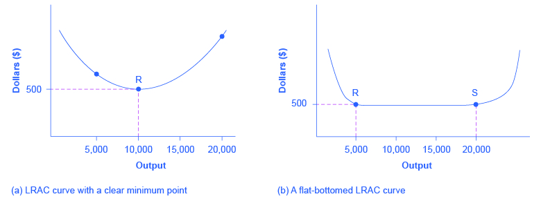
The shape of the long-run average cost curve has implications for how many firms will compete in an industry, and whether the firms in an industry have many different sizes, or tend to be the same size. For example, say that one million dishwashers are sold every year at a price of $500 each and the long-run average cost curve for dishwashers is shown in [link] (a). In [link] (a), the lowest point of the LRAC curve occurs at a quantity of 10,000 produced. Thus, the market for dishwashers will consist of 100 different manufacturing plants of this same size. If some firms built a plant that produced 5,000 dishwashers per year or 25,000 dishwashers per year, the average costs of production at such plants would be well above $500, and the firms would not be able to compete.

The lrac curve and the size and number of firms

The two graphs show how the LRAC is affected by competition between firms.
(a) Low-cost firms will produce at output level R. When the LRAC curve has a clear minimum point, then any firm producing a different quantity will have higher costs. In this case, a firm producing at a quantity of 10,000 will produce at a lower average cost than a firm producing, say, 5,000 or 20,000 units. (b) Low-cost firms will produce between output levels R and S. When the LRAC curve has a flat bottom, then firms producing at any quantity along this flat bottom can compete. In this case, any firm producing a quantity between 5,000 and 20,000 can compete effectively, although firms producing less than 5,000 or more than 20,000 would face higher average costs and be unable to compete.

Questions & Answers

Ayele, K., 2003. Introductory Economics, 3rd ed., Addis Ababa.
Widad Reply
can you send the book attached ?
Ariel
?
Ariel
What is economics
Widad Reply
the study of how humans make choices under conditions of scarcity
AI-Robot
U(x,y) = (x×y)1/2 find mu of x for y
Desalegn Reply
U(x,y) = (x×y)1/2 find mu of x for y
Desalegn
what is ecnomics
Jan Reply
this is the study of how the society manages it's scarce resources
Belonwu
what is macroeconomic
John Reply
macroeconomic is the branch of economics which studies actions, scale, activities and behaviour of the aggregate economy as a whole.
husaini
etc
husaini
difference between firm and industry
husaini Reply
what's the difference between a firm and an industry
Abdul
firm is the unit which transform inputs to output where as industry contain combination of firms with similar production 😅😅
Abdulraufu
Suppose the demand function that a firm faces shifted from Qd  120 3P to Qd  90  3P and the supply function has shifted from QS  20  2P to QS 10  2P . a) Find the effect of this change on price and quantity. b) Which of the changes in demand and supply is higher?
Toofiq Reply
explain standard reason why economic is a science
innocent Reply
factors influencing supply
Petrus Reply
what is economic.
Milan Reply
scares means__________________ends resources. unlimited
Jan
economics is a science that studies human behaviour as a relationship b/w ends and scares means which have alternative uses
Jan
calculate the profit maximizing for demand and supply
Zarshad Reply
Why qualify 28 supplies
Milan
what are explicit costs
Nomsa Reply
out-of-pocket costs for a firm, for example, payments for wages and salaries, rent, or materials
AI-Robot
concepts of supply in microeconomics
David Reply
economic overview notes
Amahle Reply
identify a demand and a supply curve
Salome Reply
i don't know
Parul
there's a difference
Aryan
Demand curve shows that how supply and others conditions affect on demand of a particular thing and what percent demand increase whith increase of supply of goods
Israr
Hi Sir please how do u calculate Cross elastic demand and income elastic demand?
Abari

Get Jobilize Job Search Mobile App in your pocket Now!

Get it on Google Play Download on the App Store Now


Source:  OpenStax, Microeconomics. OpenStax CNX. Aug 03, 2014 Download for free at http://legacy.cnx.org/content/col11627/1.10
Google Play and the Google Play logo are trademarks of Google Inc.

Notification Switch

Would you like to follow the 'Microeconomics' conversation and receive update notifications?

Ask