

| << Chapter < Page | Chapter >> Page > |
Excise taxes tend to be thought to hurt mainly the specific industries they target. For example, the medical device excise tax, in effect since 2013, has been controversial for it can delay industry profitability and therefore hamper start-ups and medical innovation. But ultimately, whether the tax burden falls mostly on the medical device industry or on the patients depends simply on the elasticity of demand and supply.
Elasticities are often lower in the short run than in the long run. On the demand side of the market, it can sometimes be difficult to change Qd in the short run, but easier in the long run. Consumption of energy is a clear example. In the short run, it is not easy for a person to make substantial changes in the energy consumption. Maybe you can carpool to work sometimes or adjust your home thermostat by a few degrees if the cost of energy rises, but that is about all. However, in the long-run you can purchase a car that gets more miles to the gallon, choose a job that is closer to where you live, buy more energy-efficient home appliances, or install more insulation in your home. As a result, the elasticity of demand for energy is somewhat inelastic in the short run, but much more elastic in the long run.
[link] is an example, based roughly on historical experience, for the responsiveness of Qd to price changes. In 1973, the price of crude oil was $12 per barrel and total consumption in the U.S. economy was 17 million barrels per day. That year, the nations who were members of the Organization of Petroleum Exporting Countries (OPEC) cut off oil exports to the United States for six months because the Arab members of OPEC disagreed with the U.S. support for Israel. OPEC did not bring exports back to their earlier levels until 1975—a policy that can be interpreted as a shift of the supply curve to the left in the U.S. petroleum market. [link] (a) and [link] (b) show the same original equilibrium point and the same identical shift of a supply curve to the left from S 0 to S 1 .
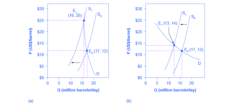
[link] (a) shows inelastic demand for oil in the short run similar to that which existed for the United States in 1973. In [link] (a), the new equilibrium (E 1 ) occurs at a price of $25 per barrel, roughly double the price before the OPEC shock, and an equilibrium quantity of 16 million barrels per day. [link] (b) shows what the outcome would have been if the U.S. demand for oil had been more elastic, a result more likely over the long term. This alternative equilibrium (E 1 ) would have resulted in a smaller price increase to $14 per barrel and larger reduction in equilibrium quantity to 13 million barrels per day. In 1983, for example, U.S. petroleum consumption was 15.3 million barrels a day, which was lower than in 1973 or 1975. U.S. petroleum consumption was down even though the U.S. economy was about one-fourth larger in 1983 than it had been in 1973. The primary reason for the lower quantity was that higher energy prices spurred conservation efforts, and after a decade of home insulation, more fuel-efficient cars, more efficient appliances and machinery, and other fuel-conserving choices, the demand curve for energy had become more elastic.
On the supply side of markets, producers of goods and services typically find it easier to expand production in the long term of several years rather than in the short run of a few months. After all, in the short run it can be costly or difficult to build a new factory, hire many new workers, or open new stores. But over a few years, all of these are possible.
Indeed, in most markets for goods and services, prices bounce up and down more than quantities in the short run, but quantities often move more than prices in the long run. The underlying reason for this pattern is that supply and demand are often inelastic in the short run, so that shifts in either demand or supply can cause a relatively greater change in prices. But since supply and demand are more elastic in the long run, the long-run movements in prices are more muted, while quantity adjusts more easily in the long run.
In the market for goods and services, quantity supplied and quantity demanded are often relatively slow to react to changes in price in the short run, but react more substantially in the long run. As a result, demand and supply often (but not always) tend to be relatively inelastic in the short run and relatively elastic in the long run. The tax incidence depends on the relative price elasticity of supply and demand. When supply is more elastic than demand, buyers bear most of the tax burden, and when demand is more elastic than supply, producers bear most of the cost of the tax. Tax revenue is larger the more inelastic the demand and supply are.
Assume that the supply of low-skilled workers is fairly elastic, but the employers’ demand for such workers is fairly inelastic. If the policy goal is to expand employment for low-skilled workers, is it better to focus on policy tools to shift the supply of unskilled labor or on tools to shift the demand for unskilled labor? What if the policy goal is to raise wages for this group? Explain your answers with supply and demand diagrams.
Notification Switch
Would you like to follow the 'Macroeconomics' conversation and receive update notifications?

|
|
|
|
|

|
|

|
|

|
|

|
|

|
|

|
|

|
|
|
|
|

|
|

|