

| << Chapter < Page | Chapter >> Page > |
The original equilibrium in the AD/AS diagram will shift to a new equilibrium if the AS or AD curve shifts. When the aggregate supply curve shifts to the right, then at every price level, a greater quantity of real GDP is produced. When the SRAS curve shifts to the left, then at every price level, a lower quantity of real GDP is produced. This module discusses two of the most important factors that can lead to shifts in the AS curve: productivity growth and input prices.
In the long run, the most important factor shifting the AS curve is productivity growth . Productivity means how much output can be produced with a given quantity of labor. One measure of this is output per worker or GDP per capita . Over time, productivity grows so that the same quantity of labor can produce more output. Historically, the real growth in GDP per capita in an advanced economy like the United States has averaged about 2% to 3% per year, but productivity growth has been faster during certain extended periods like the 1960s and the late 1990s through the early 2000s, or slower during periods like the 1970s. A higher level of productivity shifts the AS curve to the right, because with improved productivity, firms can produce a greater quantity of output at every price level. [link] (a) shows an outward shift in productivity over two time periods. The AS curve shifts out from SRAS 0 to SRAS 1 to SRAS 2 , reflecting the rise in potential GDP in this economy, and the equilibrium shifts from E 0 to E 1 to E 2 .
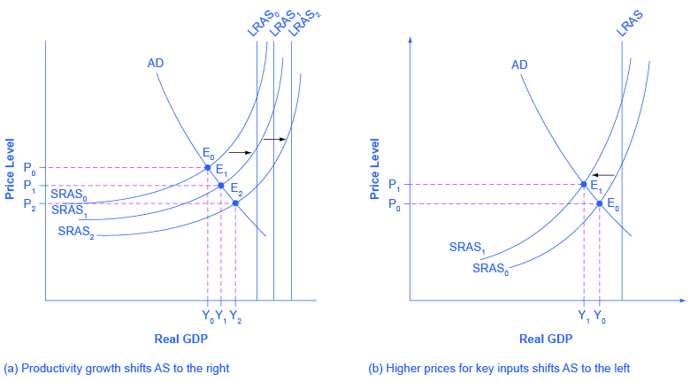
A shift in the SRAS curve to the right will result in a greater real GDP and downward pressure on the price level, if aggregate demand remains unchanged. However, if this shift in SRAS results from gains in productivity growth, which are typically measured in terms of a few percentage points per year, the effect will be relatively small over a few months or even a couple of years.
Higher prices for inputs that are widely used across the entire economy can have a macroeconomic impact on aggregate supply. Examples of such widely used inputs include wages and energy products. Increases in the price of such inputs will cause the SRAS curve to shift to the left, which means that at each given price level for outputs, a higher price for inputs will discourage production because it will reduce the possibilities for earning profits. [link] (b) shows the aggregate supply curve shifting to the left, from SRAS 0 to SRAS 1 , causing the equilibrium to move from E 0 to E 1 . The movement from the original equilibrium of E 0 to the new equilibrium of E 1 will bring a nasty set of effects: reduced GDP or recession, higher unemployment because the economy is now further away from potential GDP, and an inflationary higher price level as well. For example, the U.S. economy experienced recessions in 1974–1975, 1980–1982, 1990–91, 2001, and 2007–2009 that were each preceded or accompanied by a rise in the key input of oil prices. In the 1970s, this pattern of a shift to the left in SRAS leading to a stagnant economy with high unemployment and inflation was nicknamed stagflation .
Conversely, a decline in the price of a key input like oil will shift the SRAS curve to the right, providing an incentive for more to be produced at every given price level for outputs. From 1985 to 1986, for example, the average price of crude oil fell by almost half, from $24 a barrel to $12 a barrel. Similarly, from 1997 to 1998, the price of a barrel of crude oil dropped from $17 per barrel to $11 per barrel. In both cases, the plummeting price of oil led to a situation like that presented earlier in [link] (a), where the outward shift of SRAS to the right allowed the economy to expand, unemployment to fall, and inflation to decline.
Along with energy prices, two other key inputs that may shift the SRAS curve are the cost of labor, or wages, and the cost of imported goods that are used as inputs for other products. In these cases as well, the lesson is that lower prices for inputs cause SRAS to shift to the right, while higher prices cause it to shift back to the left.
The aggregate supply curve can also shift due to shocks to input goods or labor. For example, an unexpected early freeze could destroy a large number of agricultural crops, a shock that would shift the AS curve to the left since there would be fewer agricultural products available at any given price.
Similarly, shocks to the labor market can affect aggregate supply. An extreme example might be an overseas war that required a large number of workers to cease their ordinary production in order to go fight for their country. In this case, aggregate supply would shift to the left because there would be fewer workers available to produce goods at any given price.
The aggregate demand/aggregate supply (AD/AS) diagram shows how AD and AS interact. The intersection of the AD and AS curves shows the equilibrium output and price level in the economy. Movements of either AS or AD will result in a different equilibrium output and price level. The aggregate supply curve will shift out to the right as productivity increases. It will shift back to the left as the price of key inputs rises, and will shift out to the right if the price of key inputs falls. If the AS curve shifts back to the left, the combination of lower output, higher unemployment, and higher inflation, called stagflation, occurs. If AS shifts out to the right, a combination of lower inflation, higher output, and lower unemployment is possible.
Notification Switch
Would you like to follow the 'Macroeconomics' conversation and receive update notifications?

|
|

|
|

|
|

|
|
|
|
|

|
|

|
|

|
|

|
|

|
|

|