<< Chapter < Page Chapter >> Page >

A vertical as curve

The graph shows a straight vertical potential GDP line.
In the neoclassical model, the aggregate supply curve is drawn as a vertical line at the level of potential GDP. If AS is vertical, then it determines the level of real output, no matter where the aggregate demand curve is drawn. Over time, the LRAS curve shifts to the right as productivity increases and potential GDP expands.

The role of flexible prices

How does the macroeconomy adjust back to its level of potential GDP in the long run? What if aggregate demand increases or decreases? The neoclassical view of how the macroeconomy adjusts is based on the insight that even if wages and prices are “sticky”, or slow to change, in the short run, they are flexible over time. To understand this better, let's follow the connections from the short-run to the long-run macroeconomic equilibrium.

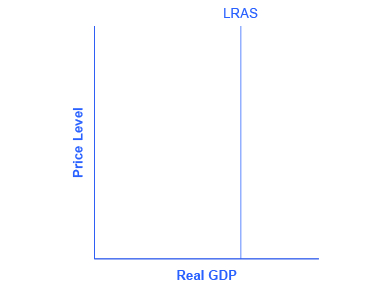
The aggregate demand and aggregate supply diagram shown in [link] shows two aggregate supply curves. The original upward sloping aggregate supply curve (SRAS 0 ) is a short-run or Keynesian AS curve. The vertical aggregate supply curve (LRASn) is the long-run or neoclassical AS curve, which is located at potential GDP. The original aggregate demand curve, labeled AD 0 , is drawn so that the original equilibrium occurs at point E 0 , at which point the economy is producing at its potential GDP.

The rebound to potential gdp after ad increases

The graph shows two aggregate demand curves and two aggregate supply curves that all intersect with the Potential GDP line at 50 on the x-axis. AD1 intersects with AS1 at point (130, 50). AD0 and AS0 intersect at point (120, 50). Additionally, AD1 intersects with AS0 at (125, 55).
The original equilibrium (E 0 ), at an output level of 500 and a price level of 120, happens at the intersection of the aggregate demand curve (AD 0 ) and the short-run aggregate supply curve (SRAS 0 ). The output at E 0 is equal to potential GDP. Aggregate demand shifts right from AD 0 to AD 1 . The new equilibrium is E 1 , with a higher output level of 550 and an increase in the price level to 125. With unemployment rates unsustainably low, wages are bid up by eager employers, which shifts short-run aggregate supply to the left, from SRAS 0 to SRAS 1 . The new equilibrium (E 2 ) is at the same original level of output, 500, but at a higher price level of 130. Thus, the long-run aggregate supply curve (LRASn), which is vertical at the level of potential GDP, determines the level of real GDP in this economy in the long run.

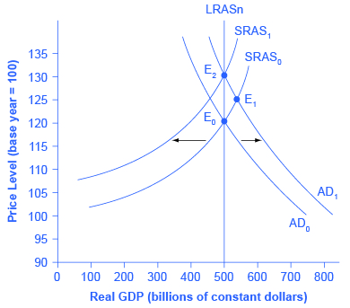
Now, imagine that some economic event boosts aggregate demand: perhaps a surge of export sales or a rise in business confidence that leads to more investment, perhaps a policy decision like higher government spending, or perhaps a tax cut that leads to additional aggregate demand. The short-run Keynesian analysis is that the rise in aggregate demand will shift the aggregate demand curve out to the right, from AD 0 to AD 1 , leading to a new equilibrium at point E 1 with higher output, lower unemployment, and pressure for an inflationary rise in the price level.

In the long-run neoclassical analysis, however, the chain of economic events is just beginning. As economic output rises above potential GDP, the level of unemployment falls. The economy is now above full employment and there is a shortage of labor. Eager employers are trying to bid workers away from other companies and to encourage their current workers to exert more effort and to put in longer hours. This high demand for labor will drive up wages. Most workers have their salaries reviewed only once or twice a year, and so it will take time before the higher wages filter through the economy. As wages do rise, it will mean a leftward shift in the short-run Keynesian aggregate supply curve back to SRAS 1 , because the price of a major input to production has increased. The economy moves to a new equilibrium (E 2 ). The new equilibrium has the same level of real GDP as did the original equilibrium (E 0 ), but there has been an inflationary increase in the price level.

Questions & Answers

Ayele, K., 2003. Introductory Economics, 3rd ed., Addis Ababa.
Widad Reply
can you send the book attached ?
Ariel
?
Ariel
What is economics
Widad Reply
the study of how humans make choices under conditions of scarcity
AI-Robot
U(x,y) = (x×y)1/2 find mu of x for y
Desalegn Reply
U(x,y) = (x×y)1/2 find mu of x for y
Desalegn
what is ecnomics
Jan Reply
this is the study of how the society manages it's scarce resources
Belonwu
what is macroeconomic
John Reply
macroeconomic is the branch of economics which studies actions, scale, activities and behaviour of the aggregate economy as a whole.
husaini
etc
husaini
difference between firm and industry
husaini Reply
what's the difference between a firm and an industry
Abdul
firm is the unit which transform inputs to output where as industry contain combination of firms with similar production 😅😅
Abdulraufu
Suppose the demand function that a firm faces shifted from Qd  120 3P to Qd  90  3P and the supply function has shifted from QS  20  2P to QS 10  2P . a) Find the effect of this change on price and quantity. b) Which of the changes in demand and supply is higher?
Toofiq Reply
explain standard reason why economic is a science
innocent Reply
factors influencing supply
Petrus Reply
what is economic.
Milan Reply
scares means__________________ends resources. unlimited
Jan
economics is a science that studies human behaviour as a relationship b/w ends and scares means which have alternative uses
Jan
calculate the profit maximizing for demand and supply
Zarshad Reply
Why qualify 28 supplies
Milan
what are explicit costs
Nomsa Reply
out-of-pocket costs for a firm, for example, payments for wages and salaries, rent, or materials
AI-Robot
concepts of supply in microeconomics
David Reply
economic overview notes
Amahle Reply
identify a demand and a supply curve
Salome Reply
i don't know
Parul
there's a difference
Aryan
Demand curve shows that how supply and others conditions affect on demand of a particular thing and what percent demand increase whith increase of supply of goods
Israr
Hi Sir please how do u calculate Cross elastic demand and income elastic demand?
Abari
Got questions? Join the online conversation and get instant answers!
Jobilize.com Reply

Get Jobilize Job Search Mobile App in your pocket Now!

Get it on Google Play Download on the App Store Now


Source:  OpenStax, Principles of economics. OpenStax CNX. Sep 19, 2014 Download for free at http://legacy.cnx.org/content/col11613/1.11
Google Play and the Google Play logo are trademarks of Google Inc.

Notification Switch

Would you like to follow the 'Principles of economics' conversation and receive update notifications?

Ask