<< Chapter < Page Chapter >> Page >

The size of these income and substitution effects will differ from person to person, depending on individual preferences. For example, if Ogden’s substitution effect away from pizza and toward haircuts is especially strong, and outweighs the income effect, then a higher price for pizza might lead to increased consumption of haircuts. This case would be drawn on the graph so that the point of tangency between the new budget constraint and the relevant indifference curve occurred below point B and to the right. Conversely, if the substitution effect away from pizza and toward haircuts is not as strong, and the income effect on is relatively stronger, then Ogden will be more likely to react to the higher price of pizza by consuming less of both goods. In this case, his optimal choice after the price change will be above and to the left of choice B on the new budget constraint.

Although the substitution and income effects are often discussed as a sequence of events, it should be remembered that they are twin components of a single cause—a change in price. Although you can analyze them separately, the two effects are always proceeding hand in hand, happening at the same time.

Indifference curves with labor-leisure and intertemporal choices

The concept of an indifference curve applies to tradeoffs in any household choice, including the labor-leisure choice or the intertemporal choice between present and future consumption. In the labor-leisure choice, each indifference curve shows the combinations of leisure and income that provide a certain level of utility. In an intertemporal choice, each indifference curve shows the combinations of present and future consumption that provide a certain level of utility. The general shapes of the indifference curves—downward sloping, steeper on the left and flatter on the right—also remain the same.

A Labor-Leisure Example

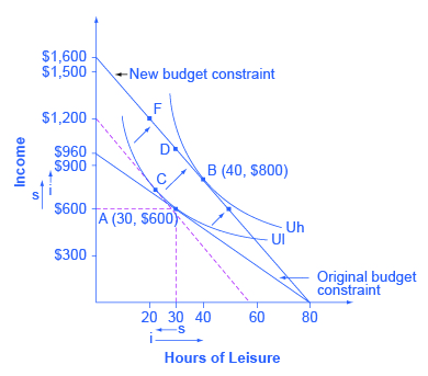
Petunia is working at a job that pays $12 per hour but she gets a raise to $20 per hour. After family responsibilities and sleep, she has 80 hours per week available for work or leisure. As shown in [link] , the highest level of utility for Petunia, on her original budget constraint, is at choice A, where it is tangent to the lower indifference curve (Ul). Point A has 30 hours of leisure and thus 50 hours per week of work, with income of $600 per week (that is, 50 hours of work at $12 per hour). Petunia then gets a raise to $20 per hour, which shifts her budget constraint to the right. Her new utility-maximizing choice occurs where the new budget constraint is tangent to the higher indifference curve Uh. At B, Petunia has 40 hours of leisure per week and works 40 hours, with income of $800 per week (that is, 40 hours of work at $20 per hour).

Effects of a change in petunia’s wage

The graph shows the effects of a change in Petunia’s wage. Petunia starts at choice A (30, $600), the tangency between her original budget constraint and the lower indifference curve Ul. The wage increase shifts her budget constraint to the right, so that she can now choose B (40, $800) on indifference curve Uh. The substitution effect is the movement from A to C which is approximately point (21, $750). In this case, the substitution effect would lead Petunia to choose less leisure, which is relatively more expensive, and more income, which is relatively cheaper to earn. The income effect is the movement from C to B.
Petunia starts at choice A, the tangency between her original budget constraint and the lower indifference curve Ul. The wage increase shifts her budget constraint to the right, so that she can now choose B on indifference curve Uh. The substitution effect is the movement from A to C. In this case, the substitution effect would lead Petunia to choose less leisure, which is relatively more expensive, and more income, which is relatively cheaper to earn. The income effect is the movement from C to B. The income effect in this example leads to greater consumption of both goods. Overall, in this example, income rises because of both substitution and income effects. However, leisure declines because of the substitution effect but increases because of the income effect—leading, in Petunia’s case, to an overall increase in the quantity of leisure consumed.

Questions & Answers

how do you get the 2/50
Abba Reply
number of sport play by 50 student construct discrete data
Aminu Reply
width of the frangebany leaves on how to write a introduction
Theresa Reply
Solve the mean of variance
Veronica Reply
Step 1: Find the mean. To find the mean, add up all the scores, then divide them by the number of scores. ... Step 2: Find each score's deviation from the mean. ... Step 3: Square each deviation from the mean. ... Step 4: Find the sum of squares. ... Step 5: Divide the sum of squares by n – 1 or N.
kenneth
what is error
Yakuba Reply
Is mistake done to something
Vutshila
Hy
anas
hy
What is the life teble
anas
hy
Jibrin
statistics is the analyzing of data
Tajudeen Reply
what is statics?
Zelalem Reply
how do you calculate mean
Gloria Reply
diveving the sum if all values
Shaynaynay
let A1,A2 and A3 events be independent,show that (A1)^c, (A2)^c and (A3)^c are independent?
Fisaye Reply
what is statistics
Akhisani Reply
data collected all over the world
Shaynaynay
construct a less than and more than table
Imad Reply
The sample of 16 students is taken. The average age in the sample was 22 years with astandard deviation of 6 years. Construct a 95% confidence interval for the age of the population.
Aschalew Reply
Bhartdarshan' is an internet-based travel agency wherein customer can see videos of the cities they plant to visit. The number of hits daily is a normally distributed random variable with a mean of 10,000 and a standard deviation of 2,400 a. what is the probability of getting more than 12,000 hits? b. what is the probability of getting fewer than 9,000 hits?
Akshay Reply
Bhartdarshan'is an internet-based travel agency wherein customer can see videos of the cities they plan to visit. The number of hits daily is a normally distributed random variable with a mean of 10,000 and a standard deviation of 2,400. a. What is the probability of getting more than 12,000 hits
Akshay
1
Bright
Sorry i want to learn more about this question
Bright
Someone help
Bright
a= 0.20233 b=0.3384
Sufiyan
a
Shaynaynay
How do I interpret level of significance?
Mohd Reply
It depends on your business problem or in Machine Learning you could use ROC- AUC cruve to decide the threshold value
Shivam
how skewness and kurtosis are used in statistics
Owen Reply
yes what is it
Taneeya
Got questions? Join the online conversation and get instant answers!
Jobilize.com Reply

Get Jobilize Job Search Mobile App in your pocket Now!

Get it on Google Play Download on the App Store Now


Source:  OpenStax, Principles of economics. OpenStax CNX. Sep 19, 2014 Download for free at http://legacy.cnx.org/content/col11613/1.11
Google Play and the Google Play logo are trademarks of Google Inc.

Notification Switch

Would you like to follow the 'Principles of economics' conversation and receive update notifications?

Ask