

| << Chapter < Page | Chapter >> Page > |
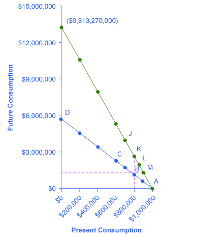
[link] and [link] show Yelberton’s intertemporal budget constraint . Yelberton’s choice involves comparing the utility of present consumption during his working life and future consumption after retirement. The rate of return that determines the slope of the intertemporal budget line between present consumption and future consumption in this example is the annual interest rate that he would earn on his savings, compounded over the 30 years of his working life. (For simplicity, we are assuming that any savings from current income will compound for 30 years.) Thus, in the lower budget constraint line on the figure, future consumption grows by increments of $574,000, because each time $100,000 is saved in the present, it compounds to $574,000 after 30 years at a 6% interest rate. If some of the numbers on the future consumption axis look bizarrely large, remember that this occurs because of the power of compound interest over substantial periods of time, and because the figure is grouping together all of Yelberton’s saving for retirement over his lifetime.
| Present Consumption | Present Savings | Future Consumption (6% annual return) | Future Consumption (9% annual return) |
|---|---|---|---|
| $1,000,000 | 0 | 0 | 0 |
| $900,000 | $100,000 | $574,000 | $1,327,000 |
| $800,000 | $200,000 | $1,148,000 | $2,654,000 |
| $700,000 | $300,000 | $1,722,000 | $3,981,000 |
| $600,000 | $400,000 | $2,296,000 | $5,308,000 |
| $400,000 | $600,000 | $3,444,000 | $7,962,000 |
| $200,000 | $800,000 | $4,592,000 | $10,616,000 |
| 0 | $1,000,000 | $5,740,000 | $13,270,000 |
Yelberton will compare the different choices along the budget constraint and choose the one that provides him with the highest utility. For example, he will compare the utility he would receive from a choice like point A, with consumption of $1 million in the present, zero savings, and zero future consumption; point B, with present consumption of $800,000, savings of $200,000, and future consumption of $1,148,000; point C, with present consumption of $600,000, savings of $400,000, and future consumption of $2,296,000; or even choice D, with present consumption of zero, savings of $1,000,000, and future consumption of $5,740,000. Yelberton will also ask himself questions like these: “Would I prefer to consume a little less in the present, save more, and have more future consumption?” or “Would I prefer to consume a little more in the present, save less, and have less future consumption?” By considering marginal changes toward more or less consumption, he can seek out the choice that will provide him with the highest level of utility.
Notification Switch
Would you like to follow the 'Principles of economics' conversation and receive update notifications?

|
|
|
|
|

|
|

|
|

|
|

|
|

|
|

|
|

|
|

|
|

|
|

|