0.4 Analog communication (Page 2/2)

Introduction to analog and Page 2 / 2

\begin{matrix} \tilde{m} (t) & = & m_{I} (t) + j m_{Q} (t) \\ \tilde{v} (t) & = & v_{I} (t) + j v_{Q} (t) \end{matrix}

yields a much simpler description of QAM:

This is a complex figure comprised of two flowcharts with various graphs below in a column format. The first column is labeled QAM modulation. The flowchart below starts with m-tilde(t), with an arrow to the right, pointing to the right at an x-circle, with an arrow to the right, pointing to the right at a box labeled Re, with an arrow to the right pointing to the right at s(t). Below the x-circle is a circle with a tilde, labeled e ^ (j 2 pi f_c t), with an arrow pointing up at the x-circle. Below this are three graphs, each with the same shape in different positions. The shape is a quadrilateral with base on the horizontal axis, two vertical sides of different length, with the right side longer than the left, and the top line segment connecting the two vertical side with a positive slope. The first graph is labeled absolute value M-tilde (f), and the shape is centered at the origin. The second is labeled absolute value m-tilde (f - f_c), and the shape is in the first quadrant only. The third is labeled absolute value S (f) and there is one shape in the first quadrant and one shape, flipped horizontally in the second quadrant. The second column is labeled QAM demodulation. The flowchart begins with r(t) with an arrow pointing to the right at an x-circle, with an arrow pointing to the right of it at a box labeled LPF, with an arrow pointing to the right at the expression v-tilde (t). Below the x-circle is a circle with a tilde, and the expression 2e ^ -(j 2 pi f_c t). Below the flowchart are three graphs with the same shapes as in the graphs in the first column. The first looks identical in shape to the third graph in the first column, except that it is labeled absolute value R(f). The second has one shape far outside in the second quadrant, one shape flipped horizontally and centered at the origin. and one large dashed trapezoid centered at the origin. It is titled absolute value R (f + f_c). The third graph has one shape centered at the origin, and is titled absolute value v-tilde(f).

Re {u (t)} = \frac{1}{2} [u (t) + u^{*} (t)] \overset{F}{\leftrightarrow} \frac{1}{2} [U (f) + U^{*} (- f)]

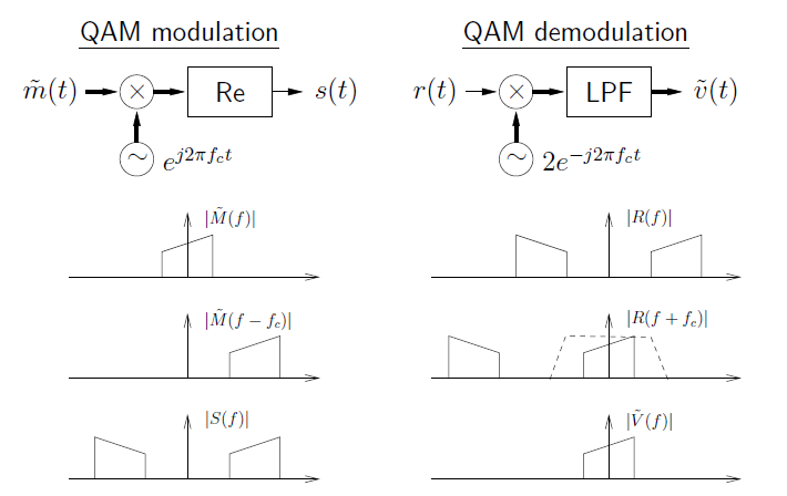
We now verify the complex-baseband model for modulation:

\begin{matrix} Re {\tilde{m} (t) e^{j 2 π f_{c} t}} \\ = & Re \{(m_{I} (t) + j m_{Q} (t)), (cos (2 π f_{c} t) + j sin (2 π f_{c} t))\} \\ = & m_{I} (t) cos (2 π f_{c} t) - m_{Q} (t) sin (2 π f_{c} t) = s (t), \end{matrix}

as well as for demodulation (assuming $r (t) = s (t)$ ):

\begin{matrix} \tilde{v} (t) & = & LPF {s (t) \cdot 2 e^{- j 2 π f_{c} t}} \\ = & LPF {(m_{I} (t) cos (2 π f_{c} t) - m_{Q} (t) sin (2 π f_{c} t)) \cdot 2 e^{- j 2 π f_{c} t}} \\ = & LPF {m_{I} (t) (e^{j 2 π f_{c} t} + e^{- j 2 π f_{c} t}) e^{- j 2 π f_{c} t} \\ - m_{Q} (t) (j e^{- j 2 π f_{c} t} - j e^{j 2 π f_{c} t}) e^{- j 2 π f_{c} t}} \\ = & LPF \{m_{I} (t) (1 + e^{- j 4 π f_{c} t}) - m_{Q} (t) (j e^{- j 4 π f_{c} t} - j)\} \\ = & m_{I} (t) + j m_{Q} (t) . \end{matrix}

The convenience of complex-baseband results in widespread use of complex-valued signals for comm systems!

To get the complex baseband formulation for AM, we simply set

m_{Q} (t) = 0

and

m_{I} (t) = m (t)

Vestigial sideband modulation (vsb)

VSB is another way to restore regain the spectral efficiency lost in AM. It's used to transmit North American terrestrial TV, both analog (NTSC)and digital (ATSC) formats.

Like AM, it can operate with or without a carrier tone.

Basically, VSB suppresses most of the redundant AM spectrum by filtering it:

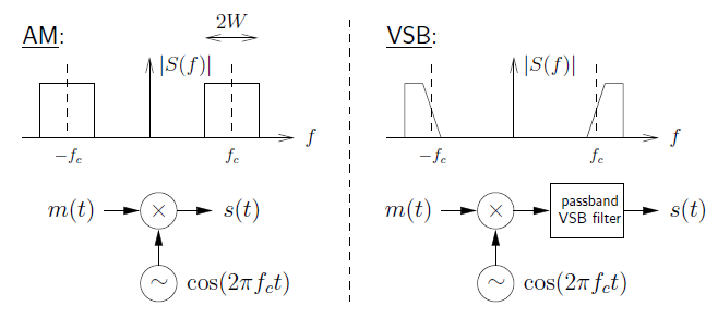
This is a two-part figure, each part containing one graph and one flowchart. The first part, on the left, is titled AM, and begins with a graph plotting f against the absolute value of S(f). There are two rectangles with vertical dashed lines in the middle, located at -f_c and f_c on the horizontal axis. Below this is a flowchart, beginning with m(t), then with an arrow pointing to the right at an x-circle, then another arrow pointing to the right at s(t). Below the x-circle is a circle with a tilde, labeled cosine (2 pi f_c t). The second part is labeled VSB. The graph plots f against the absolute value of S(f). There are two trapezoids with one vertical side and the wider base on the horizontal axis. They are also located at -f_c and f_c, and contain the vertical dashed lines in the same position as the graph in AM. Below this is a flowchart, beginning with m(t), then an arrow pointing to the right at an x-circle, then an arrow pointing to the right at a box labeled passband VSB filter, then an arrow pointing to the right at s(t). Below the x-circle is a circle with a tilde, labeled cosine (2 pi f_c t).

The passband VSB filter is a BPF $C (f)$ where

C (f - f_{c}) + C (f + f_{c}) = 2 for | f | \leq W,

which implies its inside rolloff is symmetric around $f = f_{c}$ :

This figure contains four graphs, each with vertical dashed lines at designated points and trapezoids of roughly similar shape. The first plots f against the absolute value of C(f). There are trapezoids and dashed vertical lines at -f_c and f_c. The second graph plots f against the absolute value of C(f + f_c). There are vertical dashed lines at -2f_c, -f_c, f_c, and 2f_c. There are trapezoids to the left of -2f_c and in the middle near the origin. the third graphs plots f against the absolute value of C(f - f_c), with dashed lines in the same place as in the second graph, and one trapezoid near the origin, one trapezoid near 2f_c. The fourth graph plots f against absolute value of C(f + f_c) + C(f - f_c). The vertical lines are again in the same place. There is a trapezoid at -2f_c, one at 2f_c and one larger, wider trapezoid at the origin, labeled below to be wider than 2W.

For VSB modulation, we have

\begin{matrix} s (t) & = & m (t) cos (2 π f_{c} t) * c (t) \\ S (f) & = & \frac{1}{2} [M (f + f_{c}) + M (f - f_{c})] C (f) . \end{matrix}

It turns out that VSB demod is identical to AM demod:

\begin{matrix} v (t) & = & LPF \{r (t) \cdot 2 cos (2 π f_{c} t)\} \\ = & LPF \{s (t) \cdot 2 cos (2 π f_{c} t)\} (trivial channel) \\ V (f) & = & LPF \{S (f - f_{c}) + S (f + f_{c})\} \\ = & \frac{1}{2} LPF {[M (f) + M (f - 2 f_{c})] C (f - f_{c}) \\ + [M (f + 2 f_{c}) + M (f)] C (f + f_{c})} \\ = & M (f) \underset{= 1 for f \in [- W, W]}{\underset{︸}{\frac{1}{2} [C (f - f_{c}) + C (f + f_{c})]}} \\ = & M (f) . \end{matrix}

We note that the property

\begin{matrix} F \{cos (2 π f_{c} t) c (t)\} & = & \frac{1}{2} [C (f - f_{c}) + C (f + f_{c})] \end{matrix}

may be convenient, e.g., for testing whether a given filter $c (t)$ satisfies the passband VSB criterion. VSB ﬁltering can also be implemented at baseband using a complex-valued ﬁlter response $\tilde{c} (t)$ which satisﬁes

\tilde{C} (f) + {\tilde{C}}^{*} (- f) = 2 for | f | \leq W,

generating the complex-baseband message signal $\tilde{m} (t)$ . The message can be recovered by simplying ignoring the imaginary partof the complex-baseband output $\tilde{v} (t)$ .

This figure is comprised of two columns, both beginning with a flowchart, followed by four graphs. The first column is titled VSB modulation. The flowchart shows movement from m(t) to baseband VSB flter to an x-circle with m-tilde(t) to Re to s(t), with a tilde-circle below the x-circle pointing up, labeled e^ j2πf_ct. The first graph below plots a large rectangle and a trapezoid of smaller base but same height on the graph f against the absolute value of M(f). The second graph simply shows a trapezoid with one vertical aide and same height as the shapes in the first graph, plotted this time on f against the absolute value of M-tilde(f). The third graph shows a trapezoid of the same shape, this time further into the first quadrant than the aforementioned shapes which are centered at the origin. This graph is plotted on f against the absolute value of M-tilde (f - f_c). The final graph is two trapezoids, the one on the right being identical in size and position to the trapezoid in the third graph, and the one on the left being a reflection across the vertical axis. This graph is of f plotted against the absolute value of S(f). The second column is titled VSB demodulation. The flowchart shows movement from r(t) to an x-circle to LPF, to Re by v-tilde(t), to v(t). Below the x-circle is a tilde-circle pointing up labeled 2 e^ -j2πf_ct. Below this flowchart are four graphs. The first plots f against the absolute value of R(f), and looks similar to the fourth graph in the first column. The second graph plots f against the absolute value of R(f + f_c), and it shows two trapezoids each with vertical sides on the outside, with one on the fart left, and one centered at the origin. There is also a dashed trapezoid centered at the origin that is much wider and is symmetrical. The third graph plots f against the absolute value of V-tilde(f), and simply plots one trapezoid near the origin with base on the horizontal axis and one horizontal side on the right. The final graph in this column plots f against the absolute value of V(f), and it contains a rectangle with base on the horizontal axis and centered at the origin.

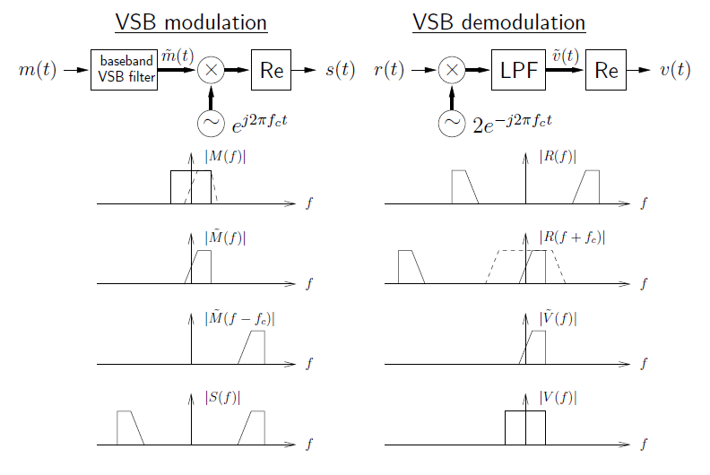
Motivation: filtering at baseband is usually much cheaper than filtering at passband.

Frequency modulation (fm)

While AM modulated the carrier amplitude, FM modulates the carrier frequency.

This figure contains three graphs each containing some waves. The first has two complete waves from horizontal value 0 to 2 with amplitude 1, and is titled message. The second plots a much larger number of waves, each with a wavelength of approximately 0.02. The amplitudes vary in a wave-like shape, increasing from nearly zero to 1, and back down to zero, and the cycle happens four times from 0 to 2. This graph is titled AM. The third graph is a series of waves of constant amplitude 1 but varying wavelength. The wavelength changes in a wave-like way and completes two cycles. This graph is titled FM.

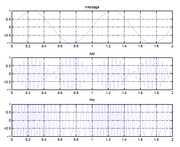
In particular, FM modulates the real-valued message $m (t)$ via

s (t) = cos (2 π f_{c} t + \underset{ϕ (t) "instantaneous modulation phase"}{\underset{︸}{2 π k_{f} \int_{0}^{t} m (τ) d τ}}) .

where $k_{f}$ is called the “frequency-sensitivity factor.” Since the instantaneous modulation frequency

\frac{d ϕ (t)}{d t} = 2 π k_{f} m (t)

is a scaled version of the message $m (t)$ , it is fitting to call this scheme “frequency modulation.”

Using the peak frequency deviation $Δ_{f} = k_{f} max | m (t) |$ , the “modulation index” D is defined as

D = \frac{Δ_{f}}{W} \begin{matrix} \leftarrow denominator is the single-sided BW of m (t) . \end{matrix}

Increasing D decreases spectral efficiency but increases robustness to noise/interference.

\begin{matrix} D ≪ 1 & : & ``narrowband FM'', \\ D ≫ 1 & : & ``wideband FM'' . \end{matrix}

Carson's Rule approximates the FM passband signal-BW as

{BW}_{99} \approx 2 (Δ_{f} + W) = 2 (D + 1) W .

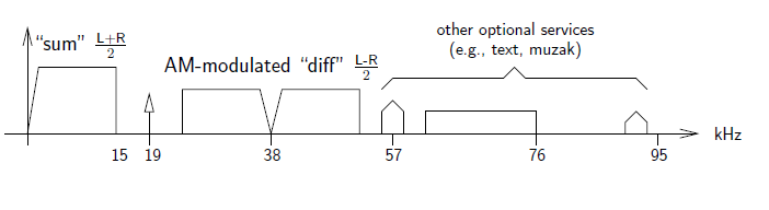
Example: Mono FM radio:

Message signal filtered to freq interval [30,15k] Hz.
FCC limits $Δ_{f} \leq 75$ kHz (channels 200 kHz apart). $\Rightarrow$ $D = \frac{75}{15} = 5$

FM stereo uses smaller D due to message spectrum:

This graph contains a number of shapes on a graph of horizontal axis kHz. The first shape is a trapezoid with a horizontal size on the right and the bottom-left vertex at the origin. The shape is titled, sum, quantity L + R divided by 2. The vertical side is located at horizontal value 15. At 19, there is a small arrow pointing up. This is followed by two trapezoids, each with vertical side on the outside, and two diagonal sides that meet at the same point on the horizontal axis, 38. These are titled AM-modulated diff, quantity L - R/2. The final group of shapes is one pentagon with horizontal base on the axis and two vertical sides, centered at value 57, another near horizontal value 95, and a rectangle with a right side at horizontal value 76. This group is titled, other optional services, text, muzak.

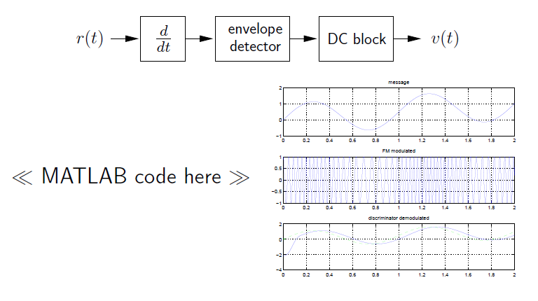
There are various FM demodulators, but the “discriminator” is one of the best known.Recalling that

\frac{d}{d t} cos (ϕ (t)) = - \frac{d ϕ (t)}{d t} sin (ϕ (t)),

we see that

\begin{matrix} \frac{d}{d t} s (t) & = & \frac{d}{d t} cos (2 π f_{c} t + 2 π k_{f} \int_{0}^{t} m (τ) d τ) \\ = & - [2 π f_{c} + 2 π k_{f} m (t)] sin (2 π f_{c} t + 2 π \int_{0}^{t} m (τ) d τ) \end{matrix}

is a form of large-carrier AM (assuming $f_{c} > k_{f} m (t)$ ), which can be demodulated using an envelope detector as follows:

This figure contains one flowchart above, and three graphs in a column to the right of a caption that reads, MATLAB code here. The flowchart shows movement from r(t) to a box labeled d/td to a box labeled envelope detector, to a box labeled DC block, to a final expression, v(t). The first graph is titled message, and is a series of waves of different amplitudes from horizontal value 0 to 2. Two full waves are completed, and their troughs and peaks are at different levels. The second graph is titled FM modulated, and consists of numerous waves of varying wavelengths. Each wave has an amplitude of 1 and the wavelengths change in a cyclical pattern. The third graph is titled discriminator demodulated, and consists of one dashed line as a wave of constant wavelength but increasing overall value, and one solid line starting with a sharp increase and continuing in a pattern that closely follows the dashed line. Two waves are completed by both lines.

<< Chapter < Page Page > Chapter >>

Read also:

Get Jobilize Job Search Mobile App in your pocket Now!

100% Free Mobile Applications
Receive real-time job alerts and never miss the right job again

Source: OpenStax, Introduction to analog and digital communications. OpenStax CNX. Sep 14, 2009 Download for free at http://cnx.org/content/col10968/1.2

Google Play and the Google Play logo are trademarks of Google Inc.

Notification Switch

Would you like to follow the 'Introduction to analog and digital communications' conversation and receive update notifications?

Ask

	4 Physiotherapy Flashcards Set 4 By Rhodes Start Flashcards
©flickr: Francisco	U.S. Civil War Pre-test By Danielle Stephens Start Quiz
©flickr:	Health Reviewer MCQ By Edgar Delgado Start Quiz
	Job Search Skills MCQ By Mary Matera Start Quiz
	Clinical Psychology MCQ By Saylor Foundation Start Quiz
	World Capitals Quiz By Yasser Ibrahim Start Quiz
	Advertising Promotion BUS210 By Melinda Salzer Start Quiz
	36 Biology 36 Sensory Systems MCQ By OpenStax Start Quiz
	1 Human A&P 2- Test 1 By Madison Christian Start Flashcards
	Engineering Communication MCQ By Steve Gibbs Start Quiz