

| << Chapter < Page | Chapter >> Page > |
We can use a direction field to predict the behavior of solutions to a differential equation without knowing the actual solution. For example, the direction field in [link] serves as a guide to the behavior of solutions to the differential equation
To use a direction field, we start by choosing any point in the field. The line segment at that point serves as a signpost telling us what direction to go from there. For example, if a solution to the differential equation passes through the point then the slope of the solution passing through that point is given by Now let increase slightly, say to Using the method of linear approximations gives a formula for the approximate value of for In particular,
Substituting into gives an approximate value of
At this point the slope of the solution changes (again according to the differential equation). We can keep progressing, recalculating the slope of the solution as we take small steps to the right, and watching the behavior of the solution. [link] shows a graph of the solution passing through the point
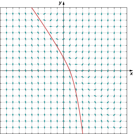
The curve is the graph of the solution to the initial-value problem
This curve is called a solution curve passing through the point The exact solution to this initial-value problem is
and the graph of this solution is identical to the curve in [link] .
Create a direction field for the differential equation and sketch a solution curve passing through the point

Go to this Java applet and this website to see more about slope fields.
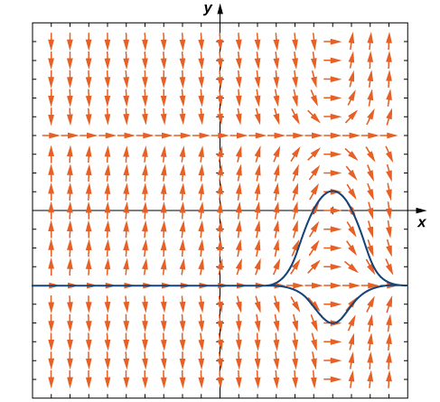
Now consider the direction field for the differential equation shown in [link] . This direction field has several interesting properties. First of all, at and horizontal dashes appear all the way across the graph. This means that if then Substituting this expression into the right-hand side of the differential equation gives
Therefore is a solution to the differential equation. Similarly, is a solution to the differential equation. These are the only constant-valued solutions to the differential equation, as we can see from the following argument. Suppose is a constant solution to the differential equation. Then Substituting this expression into the differential equation yields This equation must be true for all values of so the second factor must equal zero. This result yields the equation The solutions to this equation are and which are the constant solutions already mentioned. These are called the equilibrium solutions to the differential equation.
Notification Switch
Would you like to follow the 'Calculus volume 2' conversation and receive update notifications?

|
|

|
|

|
|

|
|

|
|

|
|

|
|
|
|
|

|
|

|