

| << Chapter < Page | Chapter >> Page > |
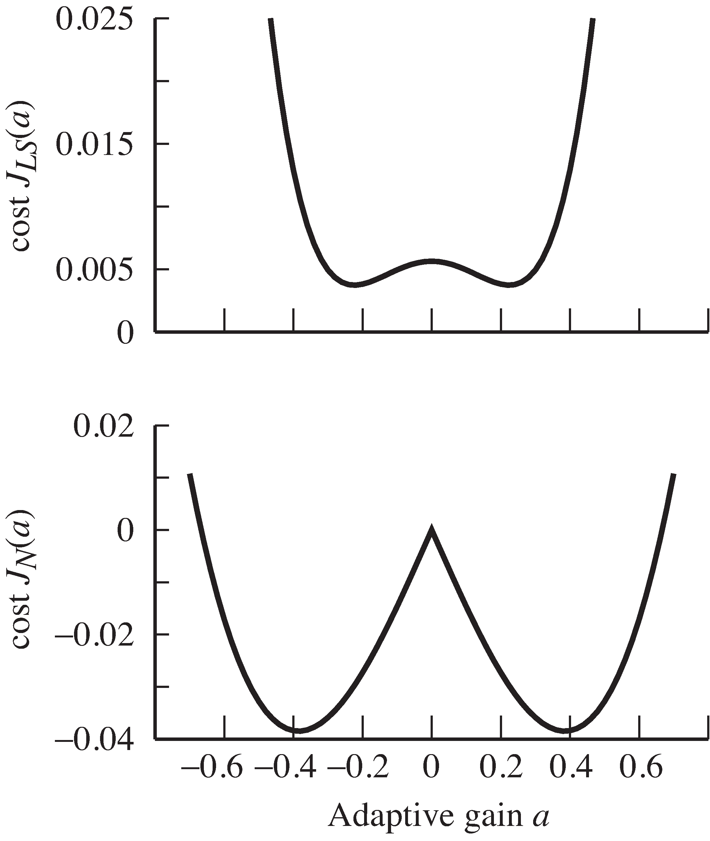
But why do the two algorithms converge to different places? The facile answer is that they are different becausethey minimize different performance functions. Indeed, the error surfaces in [link] show minima in different locations. The convergent value of for is explicable because . The convergent value of for is calculated in closed form in Exercise [link] , and this value does a good job minimizing its cost,but it has not solved the problem of making close to . Rather, calculates a smaller gain that makes . The minima are different. The moral is this:Be wary of your performance functions—they may do what you ask.
Use
agcgrad.m to investigate the AGC algorithm.
mu works?
Can the stepsize be too small?Can the stepsize be too large?mu effect the convergence
rate?a ?lenavg works?
Can
lenavg be too small?
Can
lenavg be too large?lenavg effect the convergence
rate?Show that the value of that achieves the minimum of can be expressed as
Is there a way to use this (closed form) solution to replace the iteration [link] ?
Try initializing the estimate
a(1)=-2 in
agcgrad.m .
Which minimum does the algorithm find? What happens tothe data record?
Investigate how the error surface depends on the input
signal. Replace
randn with
rand in
agcerrorsurf.m and draw the error surfaces
for both
and
.
One of the impairments encountered in transmission systems is the degradation due to fading, when the strengthof the received signal changes in response to changes in the transmission path. (Recall the discussion in [link] .) This section shows how an AGC can be used to counteractthe fading, assuming the rate of the fading is slow, and provided the signal does not disappear completely.
Suppose that the input consists of a random sequence undulating slowly up and down in magnitude, as in the topplot of [link] . The adaptive AGC compensates for the amplitude variations,growing small when the power of the input is large, and large when the power of the input is small. This is shown in themiddle graph. The resulting output is of roughly constant amplitude, as shown in the bottom plot of [link] .
Notification Switch
Would you like to follow the 'Software receiver design' conversation and receive update notifications?

|
|

|
|

|
|

|
|

|
|

|
|

|
|

|
|

|
|

|