<< Chapter < Page Chapter >> Page >

The density for the sum X + Y

Suppose the pair { X , Y } has joint density f X Y . Determine the density for

Z = X + Y

SOLUTION

F Z ( v ) = P ( X + Y v ) = P ( ( X , Y ) Q v ) where Q v = { ( t , u ) : t + u v } = { ( t , u ) : u v - t }

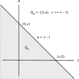
For any fixed v , the region Q v is the portion of the plane on or below the line u = v - t (see [link] ). Thus

F Z ( v ) = Q v f X Y = - - v - t f X Y ( t , u ) d u d t

Differentiating with the aid of the fundamental theorem of calculus, we get

f Z ( v ) = f X Y ( t , v - t ) d t

This integral expresssion is known as a convolution integral .
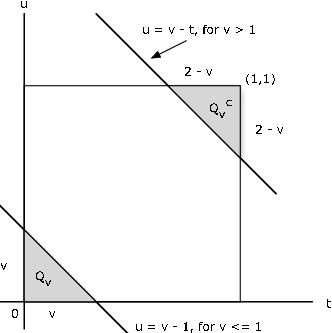
A graph of the equation Q_V{(t,u):u<=v-t}. A line ascends to the upper left intersecting the x and y axes. The area to the left of this line is shaded and the area contained on the positive side of the graph is labeled Q_V the point at which the diagonal line intersects the y axis is labeled (0,V) and where the line intersects the x axis the line is labeled (V,0). The diagonal line is labeled u=v-t A graph of the equation Q_V{(t,u):u<=v-t}. A line ascends to the upper left intersecting the x and y axes. The area to the left of this line is shaded and the area contained on the positive side of the graph is labeled Q_V the point at which the diagonal line intersects the y axis is labeled (0,V) and where the line intersects the x axis the line is labeled (V,0). The diagonal line is labeled u=v-t
Region Q v for X + Y v .
Got questions? Get instant answers now!

Sum of joint uniform random variables

Suppose the pair { X , Y } has joint uniform density on the unit square 0 t 1 , 0 u 1 . Determine the density for Z = X + Y .

SOLUTION

F Z ( v ) is the probability in the region Q v : u v - t . Now P X Y ( Q v ) = 1 - P X Y ( Q v c ) , where the complementary set Q v c is the set of points above the line. As Figure 3 shows, for v 1 , the part of Q v which has probability mass is the lower shaded triangular region on the figure, which has area (and hence probability) v 2 / 2 . For v > 1 , the complementary region Q v c is the upper shaded region. It has area ( 2 - v ) 2 / 2 . so that in this case,

P X Y ( Q v ) = 1 - ( 2 - v ) 2 / 2 . Thus,

F Z ( v ) = v 2 2 for 0 v 1 and F Z ( v ) = 1 - ( 2 - v ) 2 2 for 1 v 2

Differentiation shows that Z has the symmetric triangular distribution on [ 0 , 2 ] , since

f Z ( v ) = v for 0 v 1 and f Z ( v ) = ( 2 - v ) for 1 v 2

With the use of indicator functions, these may be combined into a single expression

f Z ( v ) = I [ 0 , 1 ] ( v ) v + I ( 1 , 2 ] ( v ) ( 2 - v )
This ia graph of the equation u=v-1, for v<=1. The x-axis is labeled t and the y-axis is labeled u. A square is formed by a line ascending from the x-axis and a line originating at the y-axis. There are two parallel line that proceed up and to the left intersecting the x and y axes for the bottom line and the two lines originating at either of the axes. These two parallel lines create two triangles. The bottom triangle contains Q_V with each one of the sides of the right angle being labeled V. The upper triangle contains Q_V^C with each of the sides of the right angle labeled 2-v and the long side being labeled u=v-t, for v > 1 This ia graph of the equation u=v-1, for v<=1. The x-axis is labeled t and the y-axis is labeled u. A square is formed by a line ascending from the x-axis and a line originating at the y-axis. There are two parallel line that proceed up and to the left intersecting the x and y axes for the bottom line and the two lines originating at either of the axes. These two parallel lines create two triangles. The bottom triangle contains Q_V with each one of the sides of the right angle being labeled V. The upper triangle contains Q_V^C with each of the sides of the right angle labeled 2-v and the long side being labeled u=v-t, for v > 1
Geometry for sum of joint uniform random variables.

ALTERNATE SOLUTION

Since f X Y ( t , u ) = I [ 0 , 1 ] ( t ) I [ 0 , 1 ] ( u ) , we have f X Y ( t , v - t ) = I [ 0 , 1 ] ( t ) I [ 0 , 1 ] ( v - t ) . Now 0 v - t 1 iff v - 1 t v , so that

f X Y ( t , v - t ) = I [ 0 , 1 ] ( v ) I [ 0 , v ] ( t ) + I ( 1 , 2 ] ( v ) I [ v - 1 , 1 ] ( t )

Integration with respect to t gives the result above.

Got questions? Get instant answers now!

Independence of functions of independent random variables

Suppose { X , Y } is an independent pair. Let Z = g ( X ) , W = h ( Y ) . Since

Z - 1 ( M ) = X - 1 [ g - 1 ( M ) ] and W - 1 ( N ) = Y - 1 [ h - 1 ( N )

the pair { Z - 1 ( M ) , W - 1 ( N ) } is independent for each pair { M , N } . Thus, the pair { Z , W } is independent.

If { X , Y } is an independent pair and Z = g ( X ) , W = h ( Y ) , then the pair { Z , W } is independent. However, if Z = g ( X , Y ) and W = h ( X , Y ) , then in general { Z , W } is not independent. This is illustrated for simple random variables with the aid of the m-procedure jointzw at the end of the next section.

Independence of simple approximations to an independent pair

Suppose { X , Y } is an independent pair with simple approximations X s and Y s as described in Distribution Approximations.

X s = i = 1 n t i I E i = i = 1 n t i I M i ( X ) and Y s = j = 1 m u j I F j = j = 1 m u j I N j ( Y )

As functions of X and Y , respectively, the pair { X s , Y s } is independent. Also each pair { I M i ( X ) , I N j ( Y ) } is independent.

Got questions? Get instant answers now!

Use of matlab on pairs of simple random variables

In the single-variable case, we use array operations on the values of X to determine a matrix of values of g ( X ) . In the two-variable case, we must use array operations on the calculating matrices t and u to obtain a matrix G whose elements are g ( t i , u j ) . To obtain the distribution for Z = g ( X , Y ) , we may use the m-function csort on G and the joint probability matrix P . A first step, then, is the use of jcalc or icalc to set up the joint distribution andthe calculating matrices. This is illustrated in the following example.

Get Jobilize Job Search Mobile App in your pocket Now!

Get it on Google Play Download on the App Store Now


Source:  OpenStax, Applied probability. OpenStax CNX. Aug 31, 2009 Download for free at http://cnx.org/content/col10708/1.6
Google Play and the Google Play logo are trademarks of Google Inc.

Notification Switch

Would you like to follow the 'Applied probability' conversation and receive update notifications?

Ask