1.4 Neural networks

Neural network implementation

For our classification task, we implement a multiclass artificial neural network. Artificial neural networks are computing structures that attempt to mimic the brain. They perform by means of distributed processing among nodes, which correspond to neurons. Connection strength between individual neurons collectively determines the network’s activity, similar to biological synapse performance. Due to the computational flexibility inherent in these large, distributed systems, neural networks excel at nonlinear tasks such as facial or speech recognition. We expected that a neural network would excel at our task: emotion classification.

Network specifications

We utilize the common multilayer perceptron neural network with neuron activation modeled by a sigmoid.

Neuron model

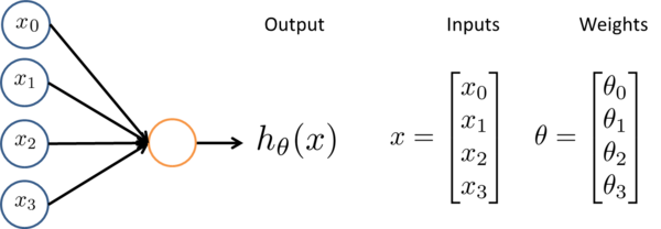
Neurons are heavily connected – one connects to many, and many to others. While each neuron takes in multiple inputs, each input is not weighted equally. The weight determines how strongly an input will affect a neuron’s output, hθ. The activation function Fa determines the relation between the inputs and the output.

The neurons of our network are characterized by the sigmoid activation function.

The sigmoid neuron has two distinct advantages. First, the sigmoid activation function is differentiable. This simplifies the function used in calculating cost for training. Second, the sigmoid activation function retains thresholding – output tends toward either 1 or 0. This enables the neurons to behave as ‘on/off’ nonlinear switches.

Network architecture

We use the same type of network as displayed in fig. 1: a multilayer perceptron. This network is feed forward, fully connected, and contains>= three layers. Feed forward means that signals travel straight through the network, from input to output, via hidden layers. No connections exist between neurons of the same layer. Fully connected means that each neuron of a previous layer has a connection between every neuron of the next layer. Feed forward systems have comparatively manageable training mechanisms, and so are preferred to other connection systems.

The input layer of a multiperceptron takes in one feature per node. The output layer contains one class per node. This layer yields the probability that an input is that particular class. The hidden layers perform operations on the inputs to yield the output. The hidden layers are thought to flesh out the distinct features that relate input to output, though what they flesh out is difficult to obtain as well as to understand.

For our application, speech features such as formant locations and power statistics are fed into 14 input nodes, and the emotion category is extracted from the 15 output nodes. The number of input nodes depends on the number of speech features, 14, that we are classifying by. The number of output nodes corresponds to the 15 emotion classes samples are categorized into. In between this input and output layer lies one hidden layer of approximately 100 artificial neurons. Our network necessitated such a large number of neurons due to the complex relation between speech features and emotion.

Training

To tailor the network for our classification task, we train its weights via feedforward-back propagation, a popular means to minimize a neural network’s cost function: J(Θ). The process is as follows:

• Randomly initialize weights between nodes. We take Θ = weight matrix.
• Implement forward propagation to determine J(Θ).

In forward propagation, all training samples are fed into the initialized neural network to obtain estimated outputs, which are used to determine J(Θ). To prevent overfitting, the cost function includes a regularization term with λ = 1, which enables control over the overall magnitudes of Θ parameters.

• Implement back propagation to determine the gradient of J(Θ). In back propagation, the error derivatives of latter layer weights are used to calculate error derivatives of former layer weights, up until all weight derivatives are found.
• Use an optimization algorithm (in our case, batch gradient descent) to minimize J(Θ), and obtain a the correct set of weights. To increase the speed of gradient descent, implement feature scaling, wherein each input feature is first shifted by the mean, and then scaled by the standard deviation.

Neural networks tend to have multiple local optima. To determine the global optima, the back propagation algorithm is run through multiple iterations (we use 1000).

Performance testing

We evaluate an independent test database with the trained neural network to test the network’s performance.

Useful references

To learn more about neural networks, check out Andrew Ng’s Machine Learning or Geoffrey Hinton’s Neural Networks for Machine learning, as found on coursera.org. Our neural network code is modified from Andrew Ng’s course code.