<< Chapter < Page Chapter >> Page >

Examples of the parks-mcclellan algorithm

Here we look at several examples of filters designed by the Parks-McClellan algorithm. The examples here are length-15 with that shown in [link] a having a passband 0 < f < 0 . 3 , a transition band 0 . 3 < f < 0 . 5 , and a stopband 0 . 5 < f < 1 . The number of cosine terms in the frequency response formula is R = 8 , therefore, the alternation theorem says we must have at least R + 1 extremal points. There are four in the passband, counting the one at zero frequency, the minimum, the maximum, andthe minimum at the bandedge. There are five in the stopband, counting the ones at the bandedge and at f = 1 . So, the number is nine which is at least R + 1 . However, in [link] c, there are ten extremal points but that is also at least 9, so it also is optimal. For a low pass filter, the maximum number of extremal points is R + 2 and that is what this filter has. This special case is called the “maximum ripple" case.

Figure two contains four graphs. The two graphs on the left side contain horizontal axes labeled Normalized frequency, numbered from 0 to 1 in increments of 0.5, and vertical axes labeled Amplitude Response, A, numbered from 0 to 1 in increments of 0.2. The top graph on the left is labeled optimal chebyshev FIR filter. The bottom graph on the left is labeled Maximum ripple chebyshev filter. Both graphs contain a curve that consists of three sections. The first section is a sinusoidal section of one complete wave centered along the vertical value of 1. These waves continue to a horizontal value of approximately 0.3. The bottom-left graph's waves have a greater amplitude than those of the top-left graph. The next section is downward sloping portion of the curve after the final peak of the first section, where it moves from approximately (0.3, 1.1) to (0.5, 0). The third section continues smoothly from the end of the second with another sinusoidal segment  with two complete waves centered about the horizontal axis. Again, the bottom-left graph's waves are larger in amplitude than the waves of the graph above. On the right, the two graphs have horizontal axes labeled real part of z, ranging in value from -2 to 2, and vertical axes labeled imaginary part of z, ranging in value from -1.5 to 1.5. Both graphs on the right consist of a circle of radius 1 centered about the origin, and various small circles at points in, on, and around the circle. The top-right graph is labeled Zero Location. On the big circle, there are eight unevenly-spaced small circles on the left half.  Beginning inside the circle, and extending outside the circle, there are five small circles that form a V-shape opening to the right. The bottom-right graph is also labeled zero location. This graph has small circles in roughly the same spots as the graph above, except that it has two extra small cirlces on the big circle, and does not contain the vertex of the v-shaped array of circles.
Amplitude Response of Length-15 Optimal Chebyshev Filters

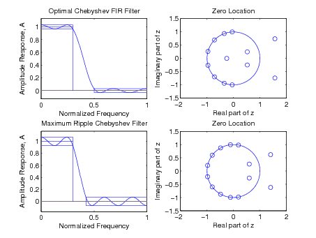
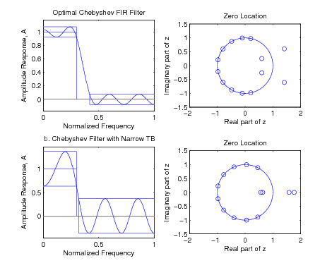
It is possible to have ripples that do not touch the maximum value and, therefore, are not considered extremal points. That is illustrated in [link] a. The effects of a narrow transitionband are illustrated in [link] c. Note the zero locations for these filters and how they relate to the amplitude response.

Figure three contains four graphs. The two graphs on the left side contain horizontal axes labeled Normalized frequency, numbered from 0 to 1 in increments of 0.5, and vertical axes labeled Amplitude Response, A, numbered from 0 to 1 in increments of 0.2. The top graph on the left is labeled optimal chebyshev FIR filter. The bottom graph on the left is labeled Chebyshev Filter with Narrow TB. Both graphs contain a curve that consists of three sections. The first section is a sinusoidal section of one complete wave centered along the vertical value of 1. These waves continue to a horizontal value of approximately 0.3. The bottom-left graph's waves have a much greater amplitude than those of the top-left graph, and only completes one-half of a wave. The next section is downward sloping portion of the curve after the final peak of the first section, where it moves from approximately (0.3, 1.1) to (0.5, 0). The third section continues smoothly from the end of the second with another sinusoidal segment  with two complete waves centered about the horizontal axis. Again, the bottom-left graph's waves are larger in amplitude than the waves of the graph above. On the right, the two graphs have horizontal axes labeled real part of z, ranging in value from -2 to 2, and vertical axes labeled imaginary part of z, ranging in value from -1.5 to 1.5. Both graphs on the right consist of a circle of radius 1 centered about the origin, and various small circles at points in, on, and around the circle. The top-right graph is labeled Zero Location. On the big circle, there are ten unevenly-spaced small circles on the left half.  Beginning inside the circle, and extending outside the circle, there are four small circles that form a V-shape opening to the right. The bottom-right graph is also labeled zero location. This graph has small circles in roughly the same spots as the graph above, except that its ten circles on the big circle are spread out over the left two-thirds. Also, instead of a v-shaped array, the graph has two small overlapping circles inside the right half of the big circle, and two small circles tangent to each other along the horizontal axis of the graph outside the big circle to the right.
Amplitude Response of Length-15 Optimal Chebyshev Filters

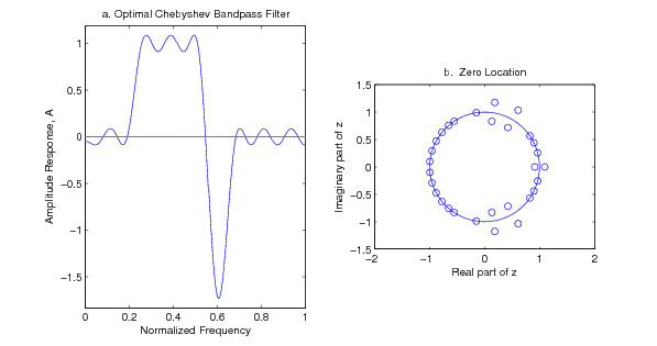
To illustrate some of the unexpected behavior that optimal filter designs can have, consider the bandpass filter amplitude response shown in [link] . Here we have a length-31 Chebyshev bandpass filter with a stopband 0 < f < 0 . 2 , a transition band 0 . 2 < f < 0 . 25 , a passband 0 . 25 < f < 0 . 5 , another transitionband 0 . 5 < f < 0 . 68 , and a stopband 0 . 68 < f < 1 . The asymmetric transition bands cause large response in the transition band around f = 0 . 6 . However, this filter is optimal since the deviation occurs in part of the frequency band that is not included in the optimization criterion. Ifyou think you don't care what happens in the transition bands, you may change your mind with this kind of behavior.

Figure four contains two graphs. Graph a is titled Optimal Chebyshev Bandpass Filter. The horizontal axis is labeled Normalized Frequency and ranges in value from 0 to 1 in increments of 0.2. The vertical axis is labeled Amplitude Response, A, and ranges in value from -1.5 to 1 in increments of 0.5. The curve begins just below the horizontal axis, first slightly downward to a small trough at approximately (0.05, -0.1). A small peak at (0.1, 0.1) follows, along with another trough at approximately (0.2, -0.1). The curve then moves sharply upward to a series of three peaks and two troughs around the vertical value 1, and horizontally from 0.2 to 0.5. After the third peak, the curve moves sharply downward to the bottom of the graph, with a trough at (0.6, -1.6). After the trough, the graph moves towards the horizontal axis and finishes with three peaks and curves of an amplitude of 0.1, then finally terminating along this pattern at the right edge of the graph. Graph b is titled Zero location. The horizontal axis is labeled Real Part of Z and ranges in value from -2 to 2 in increments of 1. The vertical axis is labeled Imaginary part of Z, and ranges in value from -1.5 to 1.5 in increments of 0.5. The graph consists of a large circle of radius 1 centered at the origin, with 30 small circles mostly falling on or around the edge of the circle. The leftmost third of the circle contains 12 of the small circles. They are closely fitted together, although not uniformly spaced, and they all are positioned on the edge of the circle. Around (0, 1) and (0, -1) are two groups of five circles, with one in each group positioned on the edge of the circle, two positioned inside the circle, and two positioned on the outside. On the rightmost third of the big circle are the remaining small circles, with all but two positioned on the edge of the big circle, and the remaining two positioned tangent to the big circle on the inside and outside around point (1, 0).
Amplitude Response of Length-31 Optimal Chebyshev Bandpass Filter

The modified parks-mcclellan algorithm

If one wants to fix the pass band ripple and minimize the stop band ripple [link] , equation [link] is changed so that the pass band ripple is added to the appropriate top part of the vector A d of the desired response and the unknown stop band is kept in the lower part of the lastcolumn of the cosine matrix C .

A d ( ω 0 ) A d ( ω 1 ) A d ( ω p ) A d ( ω s ) A d ( ω R ) + δ p - δ p ± δ p 0 0 = cos ( ω 0 0 ) cos ( ω 0 1 ) cos ( ω 0 ( R - 1 ) ) 0 cos ( ω 1 0 ) cos ( ω 1 1 ) cos ( ω 1 ( R - 1 ) ) 0 cos ( ω p 0 ) cos ( ω p 1 ) cos ( ω p ( R - 1 ) ) 0 cos ( ω s 0 ) cos ( ω s 1 ) cos ( ω s ( R - 1 ) ) 1 cos ( ω R 0 ) cos ( ω R 1 ) cos ( ω R ( R - 1 ) ) ± 1 a ( 0 ) a ( 1 ) a ( 2 ) a ( R - 1 ) δ s .

Iteration of this equation will keep the pass band ripple δ p fixed and minimize the stop band ripple δ s . A problem with convergence occurs if one of the δ 's becomes negative during the iterations. A modification to the basic exchange has been developed to give reliableconvergence [link] .

The hofstetter, oppenheim, and siegel algorithm

This algorithm [link] , [link] , [link] came into existence in order to design the filters posed by Herrmann and Schüssler [link] , [link] where both the pass and stop band ripple sizes, δ p and δ s , are fixed and the location of the transition band is not directly controlled. Thisproblem results in a maximum ripple design which, for the lowpass filter,requires extremal frequencies at both ω = 0 and ω = π but does not use either pass or stop band frequencies ω p or ω s . This results in R extremal frequencies giving R equations to find the R values of a ( n ) .

Get Jobilize Job Search Mobile App in your pocket Now!

Get it on Google Play Download on the App Store Now


Source:  OpenStax, Digital signal processing and digital filter design (draft). OpenStax CNX. Nov 17, 2012 Download for free at http://cnx.org/content/col10598/1.6
Google Play and the Google Play logo are trademarks of Google Inc.

Notification Switch

Would you like to follow the 'Digital signal processing and digital filter design (draft)' conversation and receive update notifications?

Ask