2.1 Amplitude modulation  (Page 2/4)

The am receiver (square root demodulator)

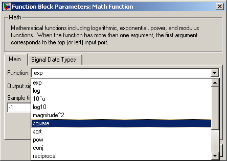
In this section you will create the model for an AM receiver based on Square Root (SQRT) demodulation. The principle of operation is shown Figure 1.

• Add the new math function block to your model. This block can be configured to implement various mathematical functions.

• Configure the block to calculate the square:

• Use the math function block to create the Square root function. You may retrieve it from the library or copy the “square” block.
• Add a digital filter design block. This block enables you to design filters using the MATLAB® FDATool.

• Configure the filter to be Low-Pass Filter. Since the carrier frequency (fc) is 15 KHz and the maximal frequency of the information is 1 KHz, the filter will be designed to pass frequencies below 5 KHz, and rejects frequencies higher than 10 KHz (please refer to Figure 16).

• Add a "Multiplier" and a "Subtract" The subtraction is created by reconfiguring the adder block, and choosing “+-“ instead of: “++” block.
• Add two "DSP Constant" blocks.
• Add the matrices concatenation object. This object will enable the modulated and the de-modulated signals to be displayed simultaneously in the scope:

• The blocks should be connected as shown in Figure 18.

• Run the simulation (push the “play” button). Double click on the scope. Scale the display to fit the scope window (Choose from the menus: Axes=>Autoscale). Choose a different color for each signal (Please refer to Figure 19).

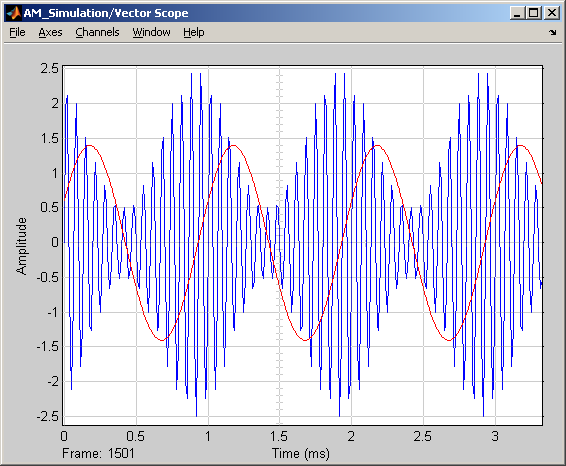
You should get the signals presented bellow:

• You may change the simulation parameters, and check their influence.

Real time implementation

The environment

The real-time implementation model will be created upon the simulation model, after the following changes:

• The signal generator block will be replaced by the CODEC of the DSK6713
• The virtual scope will be replaced also by the CODEC
• A target definition block (DSK6713) will be added.

Figure 21 shows the block-diagram for the real time implementation.

Equipment Used (shown in Figure 22):

• DSK6713
• Dual Channel Oscilloscope
• Signal Generator

We have 4 signals (4 cables):

• Information- the signal to be modulated
• Modulated- the DSK creates a modulation of the given information
• Feedback- since the transmitter and the receiver are running on the same platform, we need to perform a loopback from the transmitter to the receiver and this is exactly the feedback signal, the modulated signal that is broadcasted by the transmitter and used as input for the receiver.
• Demodulated- the signal that the receiver outputs after the demodulation process.

The procedure

• Open the model created in the previous chapter
• Remove the scope and the “information” signal (the 1,000 Hz).
• Open the Simulink library browser and add the "C6713DSK".