

| << Chapter < Page | Chapter >> Page > |
This figure was generated using the following code:
n=50000;                           % number of steps in simulation
r=randn(n,1);                      % generate raw random inputsenv=0.75+abs(sin(2*pi*[1:n]'/n));  % the fading profiler=r.*env;                          % apply profile to raw input r[k]
ds=0.5;                            % desired power of output = d^2a=zeros(1,n); a(1)=1;              % initialize AGC parameter
s=zeros(1,n);                      % initialize outputsmu=0.01;                           % algorithm stepsize
for k=1:n-1  s(k)=a(k)*r(k);                  % normalize by a(k) to get s[k]
  a(k+1)=a(k)-mu*(s(k)^2-ds);      % adaptive update of a(k)end

agcvsfading.m  compensating for fading with an AGC
(download file)
The “fading profile” defined by the vector
env is slow compared with the rate at which the adaptive gain moves,
which allows the gain to track the changes. Also, the
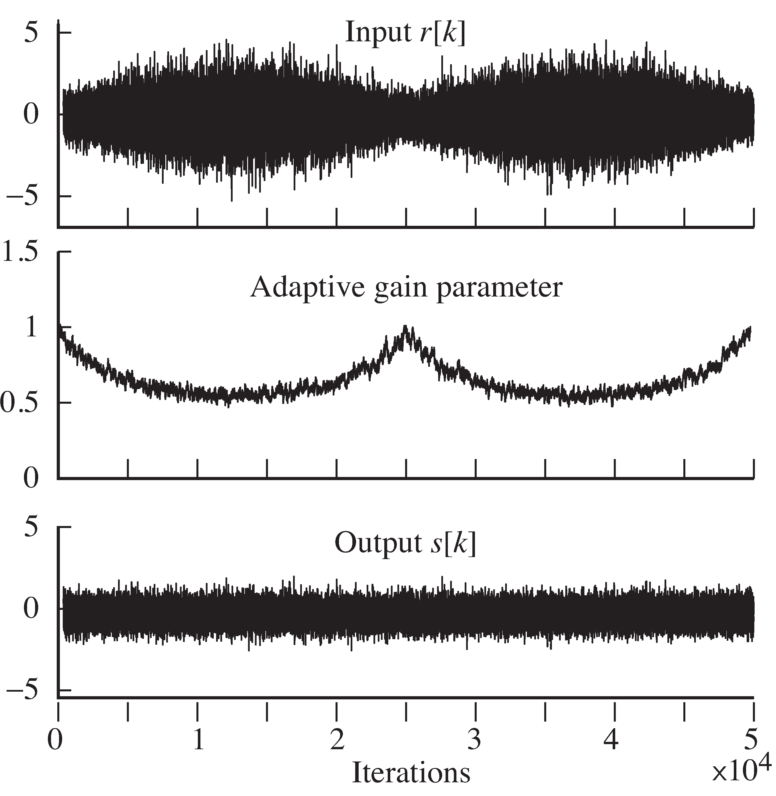
power of the input never dies away completely. The problemsthat follow ask you to investigate what happens in more extreme situations.
Mimic the code in
agcvsfading.m to
investigate what happens when the input signal diesaway. (Try removing the
abs command from the
fading profile variable.) Can you explain what you see?
Mimic the code in
agcvsfading.m to
investigate what happens when the power of the input signalvaries rapidly. What happens if the sign of the gain estimate is incorrect?
Sampling transforms a continuous-time analog signal into a discrete-time digital signal. In the time domain, thiscan be viewed as a multiplication by a train of pulses. In the frequency domain this corresponds to a replication ofthe spectrum. As long as the sampling rate is fast enough that the replicated spectra do not overlap, the samplingprocess is reversible; that is, the original analog signal can be reconstructed from the samples.
An AGC can be used to make sure that the power of the analog signal remains in the region where the sampling deviceoperates effectively. The same AGC, when adaptive, can also provide a protection against signal fades. The AGC can be designedusing a steepest descent (optimization) algorithm that updates the adaptive parameter by moving in thedirection of the negative of the derivative. This steepest descent approach to the solutionof optimization problems will be used throughout Software Receiver Design .
Details about resampling procedures are available in the published works of
which is available at his website at http://ccrma-www.stanford.edu/ jos/resample/.
A general introduction to adaptive algorithms centered around the steepest descent approach can be found in
One of our favorite discussions of adaptive methods is
This whole book can be found in .pdf form on the website accompanying this book.
Notification Switch
Would you like to follow the 'Software receiver design' conversation and receive update notifications?

|
|

|
|

|
|

|
|

|
|

|
|
|
|
|

|
|

|
|

|