0.6 Solution of the partial differential equations  (Page 13/13)

This solution is admissible in that the velocity in nondecreasing in going from the $BC$ to the $IC$ . However, it in not unique . Several values of $S2$ will give admissible solutions. Suppose that the value shown here is $\mathbf{a}$ solution. Also suppose that dispersion across the shock causes the presence of other values of $S$ between $S1$ and $S2$ . There are some values of $S$ that will have a velocity (slope) greater than that of the shock shown here. These values of $S$ will overtake $S2$ and the shock will go the these values of $S$ . This will continue until there is no value of S that has a velocity greater than that of the shock to that point. At this point the velocity of the saturation value and that of the shock are equal. On the graphic construction , the cord will be tangent to the curve at this point. This is the unique solution in the presence of a small amount of dispersion.

Composition (Saturation) Profile The composition (saturation) profile is the composition distribution existing in the system at a given time.

Composition or Flux History : The composition or flux appearing at a given point in the system, e.g., $x=1$ .

Summary of equations

The dimensionless velocity that a saturation value propagates is given by the following equation.

With uniform initial and boundary conditions, the origin of all changes in saturation is at $x=0$ and $t=0$ . If $f\left(S\right)$ depends only on $S$ and not on $x$ or $t$ , then the trajectories of constant saturation are straight line determined by integration of the above equation from the origin.

These equations give the trajectory for a given value of $S$ or for the shock. By evaluating these equations for a given value of time these equations give the saturation profile .

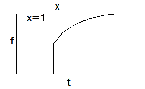
The saturation history can be determined by solving the equations for $t$ with a specified value of $x$ , e.g. $x=1$ .

The breakthrough time , $t_{BT}$ , is the time at which the fastest wave reaches $x=1.0$ . The flux history (fractional flow history) can be determined by calculating the fractional flow that corresponds to the saturation history.

Summary of diagrams

The relationship between the diagrams can be illustrated in a diagram for the trajectories. The profile is a plot of the saturation at $t=t_o$ . The history at $x=1.0$ is the saturation or fractional flow at $x=1$ . In this illustration, the shock wave is the fastest wave. Ahead of the shock is a region of constant state that is the same as the initial conditions.

New references

Carslaw, H. S. and Jaeger, J. C., Conduction of Heat in Solids, Oxford, (1959).
Churchill, R. V., Operational Mathematics, McGraw-Hill, (1958).
Courant, R. and Hilbert, D., Methods of Mathematical Physics, Volume II Partial Differential Equations, Interscience Publishers, (1962).
Hellums, J. D. and Churchill, S. W., "Mathematical Simplification of Boundary Value Problems," AIChE. J. 10, (1964) 110.
Jeffrey, A., Quasilinear Hyperbolic Systems and Waves, Pitman, (1976)
Lax, P. D., Hyperbolic System of Conservation Laws and the Mathematical Theory of Shock Waves, SIAM, (1973).
LeVeque, R. J., Numerical Methods for Conservation Laws, Birkhauser, (1992).
Milne-Thompson, L. M., Theoretical Hydrodynamics, 5th ed. Macmillan (1967).
Morse, P. M. and Feshbach, H., Methods of Theoretical Physics, (1953)
Rhee, H.-K., Aris, R., and Amundson, N. R., First-Order Partial Differential Equations: Volume I&II, Prentice-Hall (1986, 1989).