

| << Chapter < Page | Chapter >> Page > |
Listing 2 shows the constructor, which creates the raw sinusoidal data and stores that data in the array objects created in Listing 1 .
(Recall that all element values in the array objects are initialized with a value of zero. Therefore, the code in Listing 2 only needs to store the non-zero values in the array objects.)
| Listing 2. The constructor. |
|---|
public Dsp031a(){//constructor

    //Create the raw datafor(int x = 0;x<len/16;x++){
      data1[x]= amp*Math.cos(2*pi*x*freq);
    }//end for loopfor(int x = 0;x<len/8;x++){
      data2[x]= amp*Math.cos(2*pi*x*freq);
    }//end for loopfor(int x = 0;x<len/4;x++){
      data3[x]= amp*Math.cos(2*pi*x*freq);
    }//end for loopfor(int x = 0;x<len/2;x++){
      data4[x]= amp*Math.cos(2*pi*x*freq);
    }//end for loopfor(int x = 0;x<len;x++){
      data5[x]= amp*Math.cos(2*pi*x*freq);
}//end for loop}//end constructor |
The code in the conditional clause of each of the for loops in Listing 2 controls the length of each of the sinusoidal pulses.
As you can see in Listing 1 , the class implements the interface named GraphIntfc01 . I introduced this interface in the earlier module titled Plotting Engineering and Scientific Data using Java and also discussed it in the previous module titled Spectrum Analysis using Java, Sampling Frequency, Folding Frequency, and the FFT Algorithm .
The remaining code for the class named Dsp031a consists of the methods necessary to satisfy the interface. These methods are called by theplotting programs named Graph03 and Graph06 to obtain and plot the data returned by the methods. As implemented in Dsp031a , these interface methods return the values stored in the array objects referred to by data1 through data5 . Thus, the values stored in those array objects are plotted in Figure 1 .
Figure 2 shows the result of using the program named Dsp031 to perform a spectral analysis on each of the five pulses shown in Figure 1 . These results were plotted using the program named Graph06 . With this plotting program, each data value is plotted as a vertical bar.However, in this case, the sides of each of the bars are so close together that the area under the spectral curve appears to be solid black.
(When you run this program, you can expand the display to full screen and see the individual vertical bars. However, I can't do that and maintainthe narrow publication format required for this module.)
| Figure 2. Spectral analyses of five pulses. |
|---|
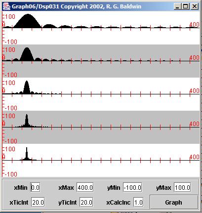 |
Before I get into the interpretation, I need to point out that I normalized the data plotted in Figure 2 to cause each spectral peak to have approximately the same value. Otherwise, the spectral analysis result values for the shortpulses would have been too small to be visible in this plotting format.
Therefore, the fact that the area under the curve in the top plot is greater than the area under the curve in the bottom plot doesn't indicate that the firstpulse contains more energy than the last pulse. It simply means that I normalized the data for best results in plotting.
Notification Switch
Would you like to follow the 'Digital signal processing - dsp' conversation and receive update notifications?

|
|
|
|
|

|
|

|
|

|
|

|
|

|
|

|
|

|
|

|