

| << Chapter < Page | Chapter >> Page > |
Both sounds and images can be considered as signals, in one or two dimensions, respectively. Sound can be described as afluctuation of the acoustic pressure in time, while images are spatial distributions of values of luminance or color, thelatter being described in its RGB or HSB components. Any signal, in order to be processed by numerical computingdevices, have to be reduced to a sequence of discrete samples , and each sample must be represented using a finite number of bits. The first operationis called sampling , and the second operation is called quantization of the domain of real numbers.
Sampling is, for one-dimensional signals, the operation that transforms a continuous-time signal (such as, for instance,the air pressure fluctuation at the entrance of the ear canal) into a discrete-time signal, that is a sequence ofnumbers. The discrete-time signal gives the values of the continuous-time signal read at intervals of seconds. The reciprocal of the sampling interval is called sampling rate . In this module we do not explain the theory of sampling, but we rather describe its manifestations. For a amore extensive yet accessible treatment, we point to the Introduction to Sound Processing . For our purposes, the process of sampling a 1-D signal canbe reduced to three facts and a theorem.
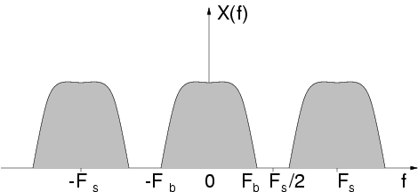
The [link] shows an example of frequency spectrum of a signal sampled with sampling rate . In the example, the continuous-time signal had all and only the frequency components between and . The replicas of the original spectrum are sometimes called images .
Given the facts , we can have an intuitive understanding of the Sampling Theorem,historically attributed to the scientists Nyquist and Shannon.
A continuous-time signal , whose spectral content is limited to frequencies smaller than (i.e., it is band-limited to ) can be recovered from its sampled version if the sampling rate is larger than twice the bandwidth (i.e., if )
Notification Switch
Would you like to follow the 'Media processing in processing' conversation and receive update notifications?

|
|

|
|

|
|

|
|

|
|

|
|

|
|
|
|
|

|
|

|