

| << Chapter < Page | Chapter >> Page > |
In this lab, we learn how to compute the continuous-time Fourier transform (CTFT), normally referred to as Fourier transform, numerically and examine its properties. Also, we explore noise cancellation and amplitude modulation as applications of Fourier transform.
In the previous labs, different mathematical transforms for processing analog or continuous-time signals were covered. Now let us explore the mathematical transforms for processing digital signals. Digital signals are sampled (discrete-time) and quantized version of analog signals. The conversion of analog-to-digital signals is implemented with an analog-to-digital (A/D) converter, and the conversion of digital-to-analog signals is implemented with a digital-to-analog (D/A) converter. In the first part of the lab, we learn how to choose an appropriate sampling frequency to achieve a proper analog-to-digital conversion. In the second part of the lab, we examine the A/D and D/A processes.
Sampling is the process of generating discrete-time samples from an analog signal. First, it is helpful to mention the relationship between analog and digital frequencies. Consider an analog sinusoidal signal . Sampling this signal at , with the sampling time interval of , generates the discrete-time signal
where denotes digital frequency with units being radians (as compared to analog frequency ω with units being radians/second).
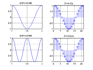
The difference between analog and digital frequencies is more evident by observing that the same discrete-time signal is obtained from different continuous-time signals if the product remains the same. (An example is shown in [link] .) Likewise, different discrete-time signals are obtained from the same analog or continuous-time signal when the sampling frequency is changed. (An example is shown in [link] .) In other words, both the frequency of an analog signal and the sampling frequency define the digital frequency of the corresponding digital signal.

It helps to understand the constraints associated with the above sampling process by examining signals in the frequency domain. The Fourier transform pairs for analog and digital signals are stated as
| Fourier transform pair for analog signals | |
| Fourier transform pair for discrete signals |

As illustrated in [link] , when an analog signal with a maximum bandwidth of (or a maximum frequency of ) is sampled at a rate of , its corresponding frequency response is repeated every radians, or . In other words, the Fourier transform in the digital domain becomes a periodic version of the Fourier transform in the analog domain. That is why, for discrete signals, one is interested only in the frequency range .
Notification Switch
Would you like to follow the 'An interactive approach to signals and systems laboratory' conversation and receive update notifications?

|
|

|
|

|
|
|
|
|

|
|

|
|

|
|
|
|
|
|
|
|
|
|