

| << Chapter < Page | Chapter >> Page > |
It costs $750 to manufacture 25 items, and $1000 to manufacture 50 items. Assuming a linear relationship holds, find the cost equation, and use this function to predict the cost of 100 items.
We let , and let .
Solving this problem is equivalent to finding an equation of a line that passes through the points (25, 750) and (50, 1000).
Therefore, the partial equation is
By substituting one of the points in the equation, we get
Therefore, the cost equation is
Now to find the cost of 100 items, we substitute in the equation
So the
The freezing temperature of water in Celsius is 0 degrees and in Fahrenheit 32 degrees. And the boiling temperatures of water in Celsius, and Fahrenheit are 100 degrees, and 212 degrees, respectively. Write a conversion equation from Celsius to Fahrenheit and use this equation to convert 30 degrees Celsius into Fahrenheit.
Let us look at what is given.
| Centigrade | Fahrenheit |
| 0 | 32 |
| 100 | 212 |
Again, solving this problem is equivalent to finding an equation of a line that passes through the points (0, 32) and (100, 212).
Since we are finding a linear relationship, we are looking for an equation , or in this case , where or represent the temperature in Celsius, and or the temperature in Fahrenheit.
The equation is
Substituting the point (0, 32), we get
Now to convert 30 degrees Celsius into Fahrenheit, we substitute in the equation
The population of Canada in the year 1970 was 18 million, and in 1986 it was 26 million. Assuming the population growth is linear, and x represents the year and y the population, write the function that gives a relationship between the time and the population. Use this equation to predict the population of Canada in 2010.
The problem can be made easier by using 1970 as the base year, that is, we choose the year 1970 as the year zero. This will mean that the year 1986 will correspond to year 16, and the year 2010 as the year 40.
Now we look at the information we have.
Solving this problem is equivalent to finding an equation of a line that passes through the points (0, 18) and (16, 26).
The equation is
Substituting the point (0, 18), we get
Now to find the population in the year 2010, we let in the equation
So the population of Canada in the year 2010 will be 38 million.
| Year | Population |
| 0 (1970) | 18 million |
| 16 (1986) | 26 million |
In this section, you will learn to:
In this section, we will do application problems that involve the intersection of lines. Therefore, before we proceed any further, we will first learn how to find the intersection of two lines.
Find the intersection of the line and the line .
We graph both lines on the same axes, as shown below, and read the solution (2, 5).
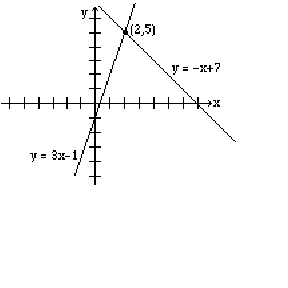
Finding an intersection of two lines graphically is not always easy or practical; therefore, we will now learn to solve these problems algebraically.
At the point where two lines intersect, the x and y values for both lines are the same. So in order to find the intersection, we either let the x-values or the y-values equal.
If we were to solve the above example algebraically, it will be easier to let the y-values equal. Since for the first line, and for the second line, by letting the y-values equal, we get
By substituting in any of the two equations, we obtain .
Hence, the solution (2, 5).
One common algebraic method used in solving systems of equations is called the elimination method . The object of this method is to eliminate one of the two variables by adding the left and right sides of the equations together. Once one variable is eliminated, we get an equation that has only one variable for which it can be solved. Finally, by substituting the value of the variable that has been found in one of the original equations, we get the value of the other variable. The method is demonstrated in the example below.
Notification Switch
Would you like to follow the 'Applied finite mathematics' conversation and receive update notifications?

|
|

|
|

|
|

|
|

|
|

|
|

|
|

|
|

|
|

|