

| << Chapter < Page | Chapter >> Page > |
Typically is a small value, say or The smaller the value of the more calculations are needed. The higher the value of the fewer calculations are needed. However, the tradeoff results in a lower degree of accuracy for larger step size, as illustrated in [link] .
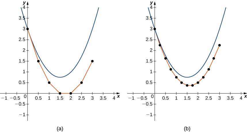
Consider the initial-value problem
Use Euler’s method with a step size of to generate a table of values for the solution for values of between and
We are given and Furthermore, the initial condition gives and Using [link] with we can generate [link] .
With ten calculations, we are able to approximate the values of the solution to the initial-value problem for values of between and
Go to this website for more information on Euler’s method.
Consider the initial-value problem
Using a step size of generate a table with approximate values for the solution to the initial-value problem for values of between and
Visit this website for a practical application of the material in this section.
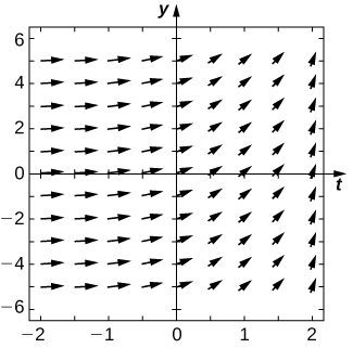
For the following problems, use the direction field below from the differential equation
Sketch the graph of the solution for the given initial conditions.
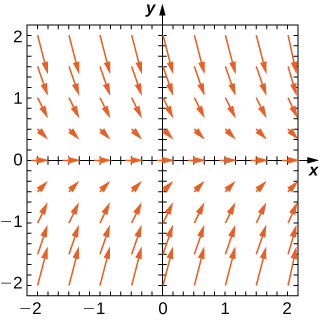
Are there any equilibria? What are their stabilities?
is a stable equilibrium
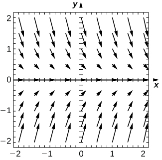
For the following problems, use the direction field below from the differential equation
Sketch the graph of the solution for the given initial conditions.

Are there any equilibria? What are their stabilities?
is a stable equilibrium and is unstable
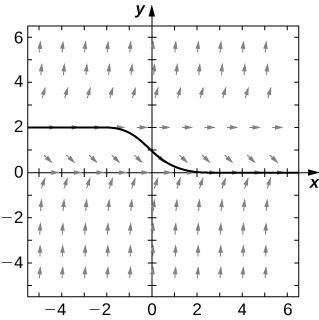
Draw the direction field for the following differential equations, then solve the differential equation. Draw your solution on top of the direction field. Does your solution follow along the arrows on your direction field?
Draw the directional field for the following differential equations. What can you say about the behavior of the solution? Are there equilibria? What stability do these equilibria have?
Notification Switch
Would you like to follow the 'Calculus volume 2' conversation and receive update notifications?

|
|

|
|

|
|

|
|
|
|
|

|
|

|
|
|
|
|

|
|

|
![A direction field over [-2, 2] in the x and y axes. The arrows point slightly down and to the right over [-2, 0] and gradually become vertical over [0, 2].](/ocw/mirror/col11965_1.2_complete/m53701/CNX_Calc_Figure_08_02_212.jpg)