<< Chapter < Page Chapter >> Page >

The design of a chebyshev lowpass filter.

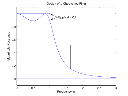
The design specifications require a maximum passband ripple of δ = 0 . 1 or a = 0 . 91515 dB, and can allow no greater response than G = 0 . 2 for frequencies above ω s = 1 . 6 radians per second.

Given δ = 0 . 1 or a = 0 . 91515 , equation [link] implies

ϵ = 0 . 484322

Given G = 0 . 2 and ω s = 1 . 6 , equation [link] implies an order of N = 3 . From ϵ and N , ν 0 is 0.49074 from [link] and

sinh ( ν 0 ) = 0 . 510675
cosh ( ν 0 ) = 1 . 122849

These multipliers are used to scale the root locations of the example third-order Butterworth filter to give

F ( s ) = 1 ( s + 0 . 51067 ) ( s + 0 . 25534 + j 0 . 97242 ) ( s + 0 . 25534 - j 0 . 97242 )
F ( s ) = 1 ( s + 0 . 51067 ) ( s 2 + 0 . 510675 s + 1 . 010789 )
F ( s ) = 1 s 3 + 102135 s 2 + 1 . 271579 s + 0 . 516185

The frequency response is shown in [link]

Figure three is a graph titled, design of a chebyshev filter. The horizontal axis is labeled Frequency, ω, and ranges in value from 0 to 3 in increments of 0.5. The vertical axis is labeled Magnitude Response and ranges in value from 0 to 1 in increments of 0.2. There is one curve on this graph. It begins at (0, 1) and decreases in a wave-like motion to a wide trough at (0.5, 0.9), and then a narrow peak at (0.9, 1). Two arrows point to the peaks and troughs and label them, ripple d = 0.1. After the peak is a large downward-sloping portion, and after a while, the curve begins to become more shallow, terminating at (3, 0).
Example Design of a Third Order Chebyshev Filter Frequency Response

Inverse-chebyshev filter properties

A second form of the mixture of a Chebyshev approximation and a Taylor's series approximation is called the Inverse Chebyshev filteror the Chebyshev II filter. This error measure uses a Taylor's series for the passband just as for the Butterworth filter and minimizes the maximumerror over the total stopband. It reverses the types of approximation usedin the preceding section. A fifth-order example is illustrated in Figure 1c from Design of Infinite Impulse Response (IIR) Filters by Frequency Transformations and [link] c.

Rather than developing the approximation directly, it is easier to modify the results from the regular Chebyshev filter. First, thefrequency variable ω in the regular Chebyshev filter, described in [link] , is replaced by 1 / ω , which interchanges the characteristics at ω equals zero and infinity and does not change the performance at ω equals unity. This converts a Chebyshev lowpass filter into a Chebyshev highpass filter as illustrated in [link] moving from the first to second frequency response.

Figure four consists of three graphs. Each graph's horizontal axis is labeled Frequency ω, and range in value from 0 to 3 in increments of 1. Each graph's vertical axis is labeled Magnitude, and ranges in value from 0 to 1 in increments of 0.2. The first graph, titled chebyshev lowpass, begins at (0, 1), and begins decreasing first as part of a wavelike segment, with two troughs and two peaks. The amplitude of the waves is approximately 0.05. By (1, 1) the second peak is reached, and the curve moves sharply downward to an eventual horizontal asymptote along the horizontal axis by (2, 0). The second, titled chebyshev highpass, begins at the origin moving horizontally for 0.5 units, then sharply increases at an increasing rate to a peak at (1, 1). After the peak, the curve quickly decreases 0.1 units to a trough, and then slowly increases to a peak at (1.7, 1), after which it slowly decreases to a nearly horizontal segment where it terminates at (3, 0.9). The third, titled inverse cheby lowpass, begins horizontally for 0.5 units from (0, 1) to (0.5, 1), where it sharply decreases to (1, 0). This point is a kink in the graph, and from this point the curve increases to a small peak at (1.3, 0.1). After the peak, the graph decreases to another kink along the horizontal axis at (1.7, 0), and then the graph finishes by increasing to a horizontal portion that terminates at (3, 0.1).
Lowpass Chebyshev to Highpass Chebyshev to Lowpass Inverse Chebyshev

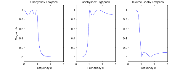
This highpass characteristic is subtracted from unity to give the desired lowpass inverse-Chebyshev frequency response illustrated in [link] c. The resulting magnitude-squared frequency- response function is given by

F F ( j ω ) = ϵ 2 C N 2 ( 1 / ω ) 1 + ϵ 2 C N 2 ( 1 / ω )

Zero locations

The zeros of the Chebyshev polynomial C N ( ω ) are easily found by

C N ( ω ) = 0 N cos - 1 ( ω ) = ( 2 k + 1 ) π / 2

which requires

ω k = cos ( ( 2 k + 1 ) π / 2 N )

for k = 0 , 1 , N - 1 , or

ω k = sin ( k π / 2 N )

for k = 0 , ± 2 , ± 4 , . . . , ± ( N - 1 ) : N odd

k = ± 1 , ± 3 , ± 5 , . . . , ± ( N - 1 ) : N even

The zeros of the inverse-Chebyshev filter transfer function are derived from [link] and [link] to give

ω z k = 1 / ( cos ( ( 2 k + 1 ) π / 2 N ) )

The zero locations are not a function of ϵ , i.e., they are independent of the stopband ripple.

Pole locations

The pole locations are the reciprocal of those for the regular Chebyshev filter. If the polesfor the inverse filter are denoted by

s k ' = σ k ' + j ω k '

the locations are

σ k ' = σ k σ k 2 + ω k 2
ω k ' = ω k σ k 2 + ω k 2

Although this gives a straightforward formula for calculating the location of the poles and zeros of the inverse-Chebyshev filter, they do not lie on a simple geometric curve as did those for the Butterworth and Chebyshev filters. Note thatthe conditions for a Taylor's series approximation with preset zero locations are satisfied.

Get Jobilize Job Search Mobile App in your pocket Now!

Get it on Google Play Download on the App Store Now


Source:  OpenStax, Digital signal processing and digital filter design (draft). OpenStax CNX. Nov 17, 2012 Download for free at http://cnx.org/content/col10598/1.6
Google Play and the Google Play logo are trademarks of Google Inc.

Notification Switch

Would you like to follow the 'Digital signal processing and digital filter design (draft)' conversation and receive update notifications?

Ask