0.8 Limitations to delay and sum beamformers

Implementing a delay and sum beamformer

As we discovered in the section discussing beamformers , that when an array of sensors record a signal there is an implicit delay between the signal arriving at the different sensors because the signal has a finite velocity and the sensors are not located at the same location in space. We can use this to our advantage, by exploiting the fact that the delay among the sensors will be different depending on which direction the signal is coming from, and tuning our array to "look" in a specific direction. This process is know as beamforming. The traditional way of beamforming is to calculate how much delay there will be among the sensors for sound coming from a direction that you are interested in. Once you know this delay you can delay all the corresponding channels the correct amount and add the signals from all the channels. In this way, you will constructively reinforce the signal that you are interested in, while signals from other directions will be out of phase and will not be reinforced.

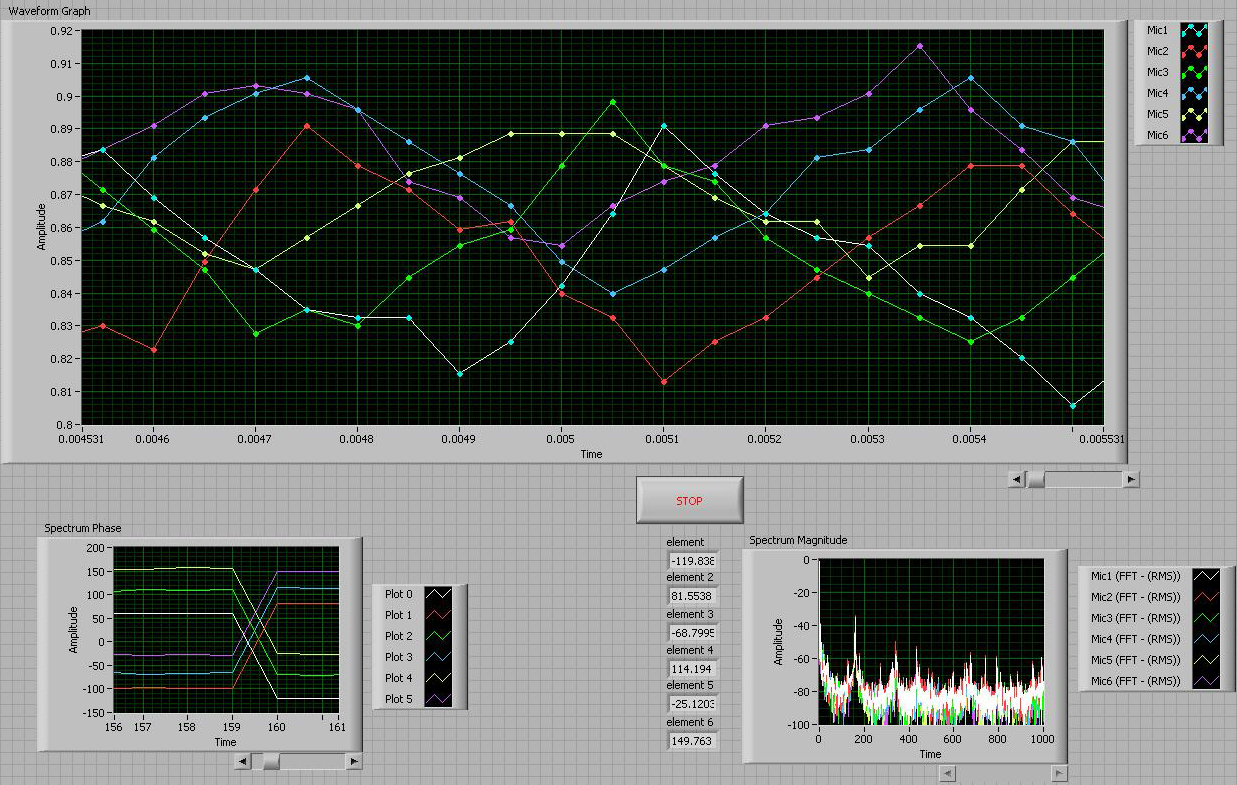
The figure above illustrates a sinusoid captured on a six channel linear array. Though, the sinusoids look crude because of the implicit noise of real signals, you can see by the spectrum that it is indeed there and in also that the phase is different for each of the sensors. The phase difference is determined by the delay between the sensors and is given by a simple geometrical calculation which we discuss later.

The problem with this method is that the degree of resolution that you can distinguish is determined by the sampling rate of your data, because you can not resolve delay differences less than your sampling rate. For example if the sampling period is 3 milliseconds, then you would have a range of say 20 degrees where the delay would be less than 3 milliseconds, and thus they would all appear to be coming from the same direction because digitizing signals from anywhere in this range would result in the same signal.

This is very significant because the spacing of the sensors is usually quite small, on the order of centimeters. At the average rate of sound, 330 m/s, it only takes .3 milliseconds to move 10 cm. However, the Nyquist Sampling Theorem states that we can derive all the information about a signal by sampling at only twice the highest frequency contained in the signal. With a 10 cm spacing between sensors the highest sinusoid we can capture is 1600 Hz, for reasons we discuss elsewhere. So ,we should be able determine the phase of all the sinusoids by only sampling at 3200 Hz rather than at tens of kilohertz that is required with delay and sum beamforming. In order to do this, however, we must implement a better method of beamforming in the frequency domain.