0.4 Streaming fft  (Page 10/19)

The only other difference when $VL>1$ is that the registers need to be transposed before storing columns to rows (the implicit transpose that corresponds to step 3). To accomplish this when generating code, $n=VL$ store operations are latched before the transpose and store code is emitted.

Example

[link] implements a VL-2 size-64 hard-coded four-step FFT. The main function (line 39) computes 8 FFTs along the columns for step 1 at line 44, and 8 FFTs along the columns for step 4 at line 45. There are only 4 iterations of the loop in each case because two sub-transforms are computed in parallel with each invocation of the sub-transform function.

In the function corresponding to the sub-transforms of step 1 (line 3), two store operations are latched (lines 23 and 24) before emitting code, which includes the preceding transposes (the TX2 operations) and twiddle factor multiplications (lines 13–22).

Performance

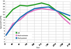
[link] shows the results of a benchmark for transforms of size 16 through to 8192 running on a Macbook Air 4,2. The speed of FFTW 3.3 running in estimate and patient modes is also shown for contrast.

The results show that the performance of the four-step algorithm improves as the length of the vector increases, but, as was the case with the hard-coded FFTs in "Fully hard-coded" , the performance of the hard-coded four-step FFTs is limited to a certain range of transform size.

Hard-coded leaves

The performance of the fully hard-coded transforms presented in "Fully hard-coded" only scales while $N/VL\le 128$ . This section presents techniques that are similar to those found in the fully hard-coded transforms, but applied at another level of scale in order to scale performance to larger sizes.

Vector length 1

The fully hard-coded transforms in "Fully hard-coded" used two primitives at the leaves: a size-4 sub-transform ( L_4 ) and a double size-2 sub-transform ( L_2 ). These sub-transforms loaded four elements of data from the input array, performed a small amount of computation, and stored the four results to the output array.

Performance is scaled to larger transforms by using larger sub-transforms at the leaves of the computation. These are automatically generated using fully hard-coded transforms, and thus the size of the leaf computations is easily parametrized, which is just as well, because the optimal leaf size is dependent on the size of the transform, the compiler, and the target machine.

The process of elaborating a topological ordering of nodes representing a hard-coded leaf transform of size $N$ with leaf sub-transforms of size $N_{leaf}$ is as follows:

1. Elaborate a size $N_{leaf}$ sub-transform;
2. Elaborate a two size $N_{leaf}/2$ sub-transforms as one sub-transform;
3. Elaborate the main transform using the sub-transforms from steps 1 and 2 as the leaves of the computation.

The node lists for steps 1 and 2 are elaborated using the fully hard-coded elaborate function from [link] , but because the leaf sub-transform in step 2 is actually two sub-transforms of size $N_{leaf}/2$ , the elaborate function is invoked twice with different offset parameters: