

| << Chapter < Page | Chapter >> Page > |
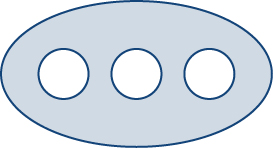
Green’s theorem, as stated, applies only to regions that are simply connected—that is, Green’s theorem as stated so far cannot handle regions with holes. Here, we extend Green’s theorem so that it does work on regions with finitely many holes ( [link] ).
Before discussing extensions of Green’s theorem, we need to go over some terminology regarding the boundary of a region. Let D be a region and let C be a component of the boundary of D . We say that C is positively oriented if, as we walk along C in the direction of orientation, region D is always on our left. Therefore, the counterclockwise orientation of the boundary of a disk is a positive orientation, for example. Curve C is negatively oriented if, as we walk along C in the direction of orientation, region D is always on our right. The clockwise orientation of the boundary of a disk is a negative orientation, for example.
Let D be a region with finitely many holes (so that D has finitely many boundary curves), and denote the boundary of D by ( [link] ). To extend Green’s theorem so it can handle D , we divide region D into two regions, and (with respective boundaries and in such a way that and neither nor has any holes ( [link] ).
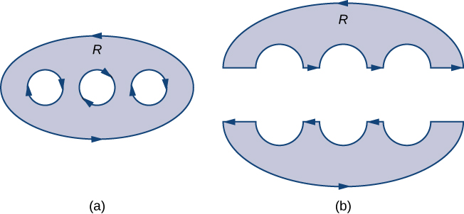
Assume the boundary of D is oriented as in the figure, with the inner holes given a negative orientation and the outer boundary given a positive orientation. The boundary of each simply connected region and is positively oriented. If F is a vector field defined on D , then Green’s theorem says that
Therefore, Green’s theorem still works on a region with holes.
To see how this works in practice, consider annulus D in [link] and suppose that is a vector field defined on this annulus. Region D has a hole, so it is not simply connected. Orient the outer circle of the annulus counterclockwise and the inner circle clockwise ( [link] ) so that, when we divide the region into and we are able to keep the region on our left as we walk along a path that traverses the boundary. Let be the upper half of the annulus and be the lower half. Neither of these regions has holes, so we have divided D into two simply connected regions.
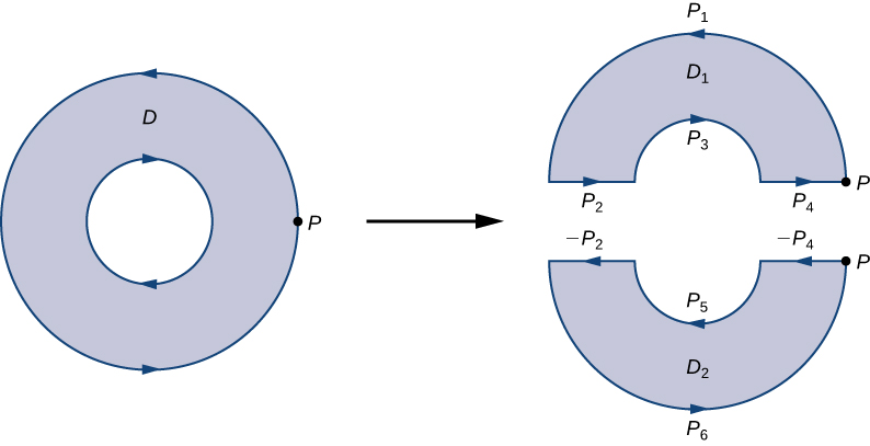
We label each piece of these new boundaries as for some i, as in [link] . If we begin at P and travel along the oriented boundary, the first segment is then and Now we have traversed and returned to P. Next, we start at P again and traverse Since the first piece of the boundary is the same as in but oriented in the opposite direction, the first piece of is Next, we have then and finally
[link] shows a path that traverses the boundary of D . Notice that this path traverses the boundary of region returns to the starting point, and then traverses the boundary of region Furthermore, as we walk along the path, the region is always on our left. Notice that this traversal of the paths covers the entire boundary of region D. If we had only traversed one portion of the boundary of D , then we cannot apply Green’s theorem to D .
Notification Switch
Would you like to follow the 'Calculus volume 3' conversation and receive update notifications?

|
|

|
|

|
|

|
|

|
|

|
|

|
|

|
|

|
|

|