<< Chapter < Page Chapter >> Page >
This module describes how to graph basic functions.

Graphing, like algebraic generalizations, is a difficult topic because many students know how to do it but are not sure what it means .

For instance, consider the following graph:
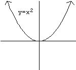
A parabola showing the graph of y=x-squared

If I asked you “Draw the graph of y = x 2 size 12{y=x rSup { size 8{2} } } {} ” you would probably remember how to plot points and draw the shape.

But suppose I asked you this instead: “Here’s a function, y = x 2 size 12{y=x rSup { size 8{2} } } {} . And here’s a shape, that sort of looks like a U. What do they actually have to do with each other?” This is a harder question! What does it mean to graph a function?

The answer is simple, but it has important implications for a proper understanding of functions. Recall that every point on the plane is designated by a unique ( x , y ) size 12{ \( x,y \) } {} pair of coordinates: for instance, one point is ( 5,3 ) size 12{ \( 5,3 \) } {} . We say that its x size 12{x} {} -value is 5 and its y size 12{y} {} -value is 3.

A few of these points have the particular property that their y size 12{y} {} -values are the square of their x size 12{x} {} -values. For instance, the points ( 0,0 ) size 12{ \( 0,0 \) } {} , ( 3,9 ) size 12{ \( 3,9 \) } {} , and ( 5, 25 ) size 12{ \( - 5, 25 \) } {} all have that property. ( 5,3 ) size 12{ \( 5,3 \) } {} and ( 2, 4 ) size 12{ \( - 2, - 4 \) } {} do not.

The graph shown—the pseudo-U shape—is all the points in the plane that have this property . Any point whose y size 12{x} {} -value is the square of its x size 12{x} {} -value is on this shape; any point whose y size 12{y} {} -value is not the square of its x size 12{x} {} -value is not on this shape. Hence, glancing at this shape gives us a complete visual picture of the function y = x 2 size 12{y=x rSup { size 8{2} } } {} if we know how to interpret it correctly .

Graphing functions

Remember that every function specifies a relationship between two variables. When we graph a function, we put the independent variable on the x size 12{x} {} -axis, and the dependent variable on the y size 12{y} {} -axis.

For instance, recall the function that describes Alice’s money as a function of her hours worked. Since Alice makes $12/hour, her financial function is m ( t ) = 12 t size 12{m \( t \) ="12"t} {} . We can graph it like this.

a graph depicting the function of Alice's pay.

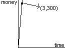
This simple graph has a great deal to tell us about Alice’s job, if we read it correctly.

  • The graph contains the point ( 3, 300 ) size 12{ \( 3,"300" \) } {} .What does that tell us? That after Alice has worked for three hours, she has made $300.
  • The graph goes through the origin (the point ( 0,0 ) size 12{ \( 0,0 \) } {} ). What does that tell us? That when she works 0 hours, Alice makes no money.
  • The graph exists only in the first quadrant. What does that tell us? On the mathematical level, it indicates the domain of the function ( t 0 size 12{t>= 0} {} ) and the range of the function ( m 0 size 12{m>= 0} {} ). In terms of the situation, it tells us that Alice cannot work negative hours or make negative money.
  • The graph is a straight line. What does that tell us? That Alice makes the same amount of money every day: every day, her money goes up by $100. ($100/day is the slope of the line—more on this in the section on linear functions.)

Consider now the following, more complicated graph, which represents Alice’s hair length as a function of time (where time is now measured in weeks instead of hours).
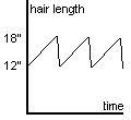
A right slanted saw-tooth graph oscillating between 12 and 18 inches.

What does this graph h ( t ) size 12{h \( t \) } {} tell us? We can start with the same sort of simple analysis.

  • The graph goes through the point ( 0, 12 ) size 12{ \( 0,"12" \) } {} .This tells us that at time ( t = 0 ) size 12{ \( t=0 \) } {} , Alice’s hair is 12" long.
  • The range of this graph appears to be 12 h 18 size 12{"12"<= h<= "18"} {} . Alice never allows her hair to be shorter than 12" or longer than 18".

Get Jobilize Job Search Mobile App in your pocket Now!

Get it on Google Play Download on the App Store Now


Source:  OpenStax, Advanced algebra ii: conceptual explanations. OpenStax CNX. May 04, 2010 Download for free at http://cnx.org/content/col10624/1.15
Google Play and the Google Play logo are trademarks of Google Inc.

Notification Switch

Would you like to follow the 'Advanced algebra ii: conceptual explanations' conversation and receive update notifications?

Ask