

| << Chapter < Page | Chapter >> Page > |
To make our discussion of SVMs easier, we'll first need to introduce a new notation for talking about classification.We will be considering a linear classifier for a binary classification problem with labels and features . From now, we'll use (instead of ) to denote the class labels. Also, rather than parameterizing our linearclassifier with the vector , we will use parameters , and write our classifier as
Here, if , and otherwise. This “ ” notation allows us to explicitly treat the intercept term separately from the other parameters. (We also drop the convention we had previously of letting be an extra coordinate in the input feature vector.) Thus, takes the role of what was previously , and takes the role of .
Note also that, from our definition of above, our classifier will directly predict either 1 or (cf. the perceptron algorithm), without first going through the intermediate step of estimating the probability of being 1 (which was what logistic regression did).
Let's formalize the notions of the functional and geometric margins. Given a training example , we define the functional margin of with respect to the training example
Note that if , then for the functional margin to be large (i.e., for our prediction to be confident and correct), we need to be a large positive number. Conversely, if , then for the functional margin to be large, we need to be a large negative number. Moreover, if , then our prediction on this example is correct. (Check this yourself.)Hence, a large functional margin represents a confident and a correct prediction.
For a linear classifier with the choice of given above (taking values in ), there's one property of the functional margin that makes it not a very good measure of confidence,however. Given our choice of , we note that if we replace with and with , then since , this would not change at all. I.e., , and hence also , depends only on the sign, but not on the magnitude, of . However, replacing with also results in multiplying our functional margin by a factor of 2. Thus, it seems that by exploiting our freedom to scale and , we can make the functional margin arbitrarily large without really changing anything meaningful. Intuitively, it might therefore make senseto impose some sort of normalization condition such as that ; i.e., we might replace with , and instead consider the functional margin of . We'll come back to this later.
Given a training set , we also define the function margin of with respect to to be the smallest of the functional margins of the individual training examples. Denotedby , this can therefore be written:
Next, let's talk about geometric margins . Consider the picture below:
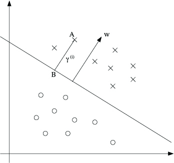
The decision boundary corresponding to is shown, along with the vector . Note that is orthogonal (at ) to the separating hyperplane. (You should convince yourself that this must be the case.) Consider the point at A, which represents the input of some training example with label . Its distance to the decision boundary, , is given by the line segment AB.
Notification Switch
Would you like to follow the 'Machine learning' conversation and receive update notifications?

|
|

|
|

|
|

|
|

|
|

|
|

|
|

|
|

|
|

|