which algorithm to run: trained LMS, decision-directed LMS, or
blind DMA,
the stepsize, and
the initialization: a scale factor specifies the
size of the ball about the optimum equalizer within which theinitial value for the equalizer is randomly chosen
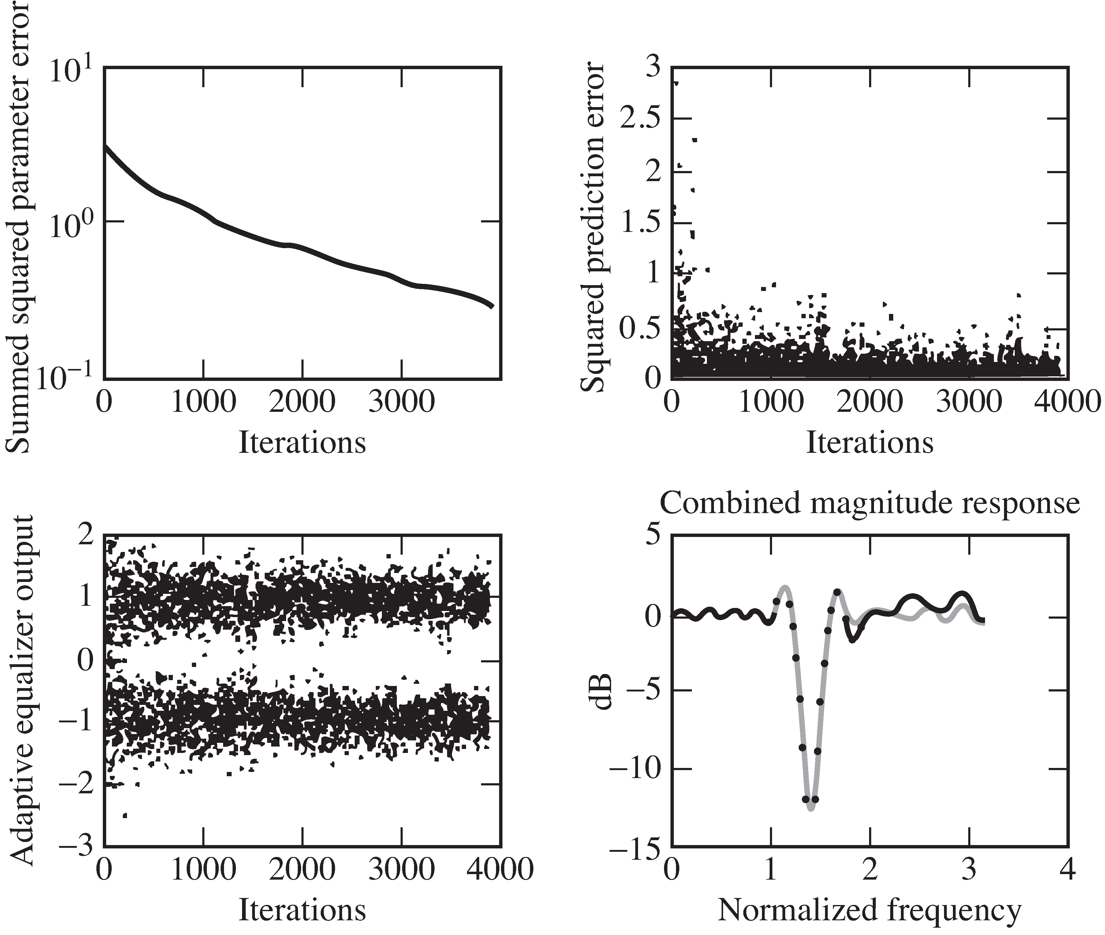
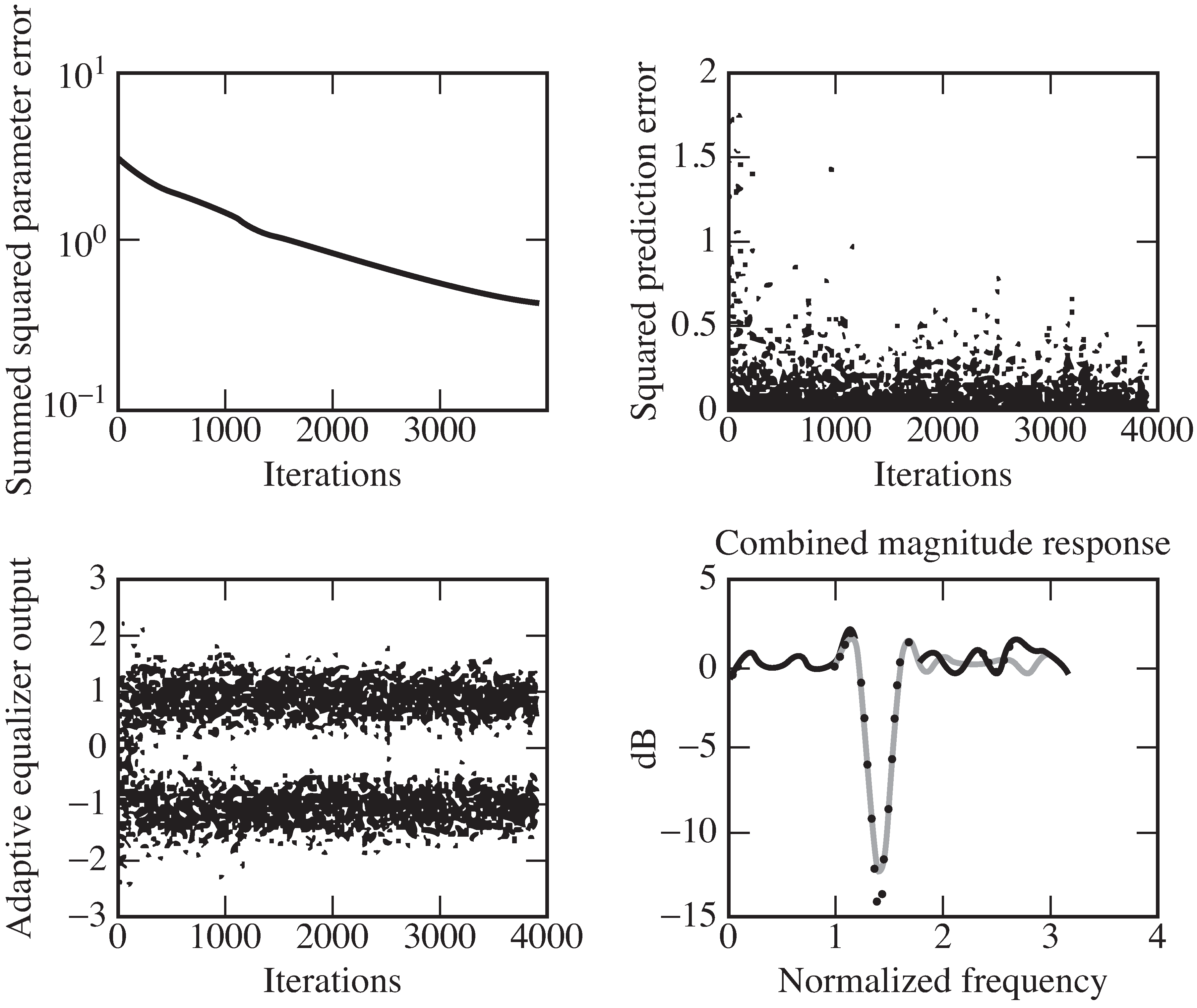
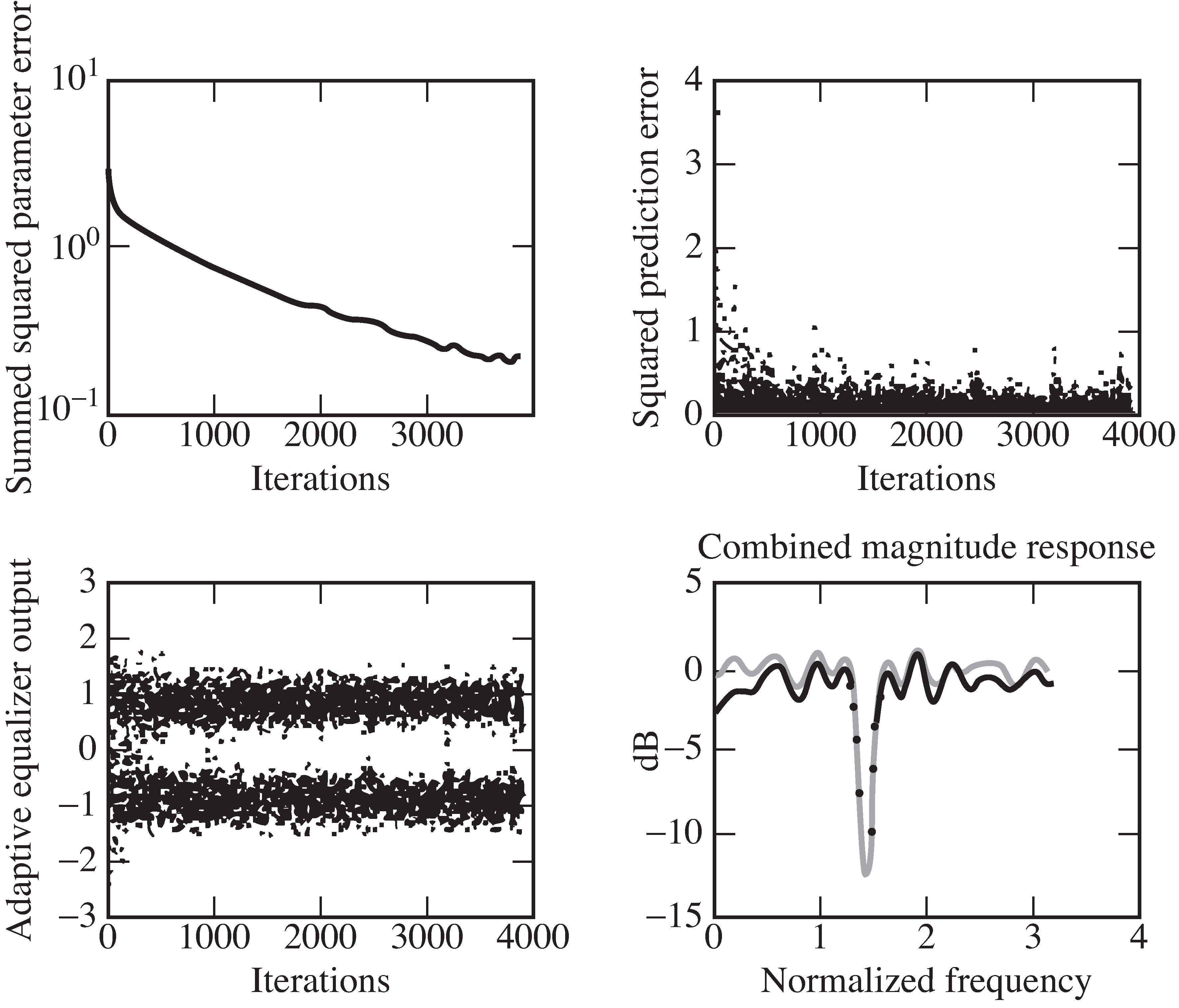
As is apparent from
[link] –
[link] ,
all three adaptive schemes are successful with the recommended “default”values, which were used in equalizing channel 0.
All three exhibit, in the upper left plotsof
[link] -
[link] ,
decaying averaged squared parameter error relativeto their respective trained least-squares equalizer for the data block.
This means that all are converging to the vicinity of thetrained least-squares equalizer about which
dae.m initializes the algorithms.
The collapse of the squared prediction error is apparent from theupper right plot in each of the same figures.
An initially closed eye appears for a short while ineach of the lower left plots of equalizer output history
in the same figures.The match of the magnitudes of the
frequency responses of the trained (block) least-squaresequalizer (plotted with the solid line)
and the last adaptive equalizer setting(plotted with asterisks) from the data block
stream is quite striking in the lower right plotsin the same figures.
As expected,
With modest noise, as in the cases
here outside the frequency band occupied by the single narrowband interferer, the magnitude of the frequency responseof the trained least-squares
solution exhibits peaks (valleys)where the channel response has valleys (peaks)
so that the combined response is nearly flat.The phase of the trained least-squares equalizer
adds with the channel phase so that their combinationapproximates a linear phase curve.
Refer to plots in the right columns of
[link] ,
[link] , and
[link] .
With modest channel noise and interferers,
as the length of the equalizer increases,
the zeros of the combined channel and equalizer form rings.The rings are denser the nearer the channel zeros are to the
unit circle.
There are many ways that the program
dae.m can be used
to investigate and learn about equalization.Try to choose the various parameters to observe that
Increasing the power of the channel noise suppresses the
frequency response of the least-squares equalizer,with those frequency bands most suppressed being those
in which the channel has a null (and theequalizer—without channel noise—would have a peak).
Trained LMS equalizer for Channel 0.
The *** represents the achieved frequency response of theequalizer while the solid line represents the frequency response
of the desired (optimal) mean square error solution.Decision-directed LMS equalizer for Channel 0.
The *** represents the achieved frequency response of theequalizer while the solid line represents the frequency response
of the desired (optimal) mean square error solution.Blind DMA equalizer for Channel 0.
The *** represents the achieved frequency response of theequalizer while the solid line represents the frequency response
of the desired (optimal) mean square error solution.
Increasing the gain of a narrowband interferer results in a
deepening of a notch in the trained least squaresequalizer at the frequency of the interferer.
DMA is considered slower than trained LMS.
Do you find that DMA takes longer to converge?Can you think of why it might be slower?
DMA typically accommodates larger initialization error than
decision-directed LMS. Can you find cases where, with thesame initialization, DMA converges to an error-free solution
but the decision directed LMS does not? Do you think thereare cases in which the opposite holds?
It is necessary to specify the delay
for the
trained LMS, whereas the blind methods do not requirethe parameter
. Rather, the selection of an
appropriate delay is implicit in the initialization of theequalizer coefficients.
Can you find a case in which,with the delay poorly specified, DMA outperforms
trained LMS from the same initialization?
For further reading
A comprehensive survey of trained adaptive equalization
can be found in
S. U. H. Qureshi, “Adaptive equalization,”
Proceedings of the IEEE , pp. 1349–1387, 1985.
An overview of the analytical tools that can be used to
analyze LMS-style adaptive algorithms can be found in
W. A. Sethares, “The LMS Family,” in
Efficient System
Identification and Signal Processing Algorithms ,
Ed. N. Kalouptsidis and S. Theodoridis, Prentice Hall, 1993.
A copy of this paper can also be found on the accompanying website.
One of our favorite discussions of adaptive methods is
C. R. Johnson Jr.,
Lectures on Adaptive Parameter Estimation, Prentice-Hall,
1988.
This whole book can be found in .pdf form on the website.
An extensive discussion of equalization can also be
found in
Equalization on the website.