

| << Chapter < Page | Chapter >> Page > |
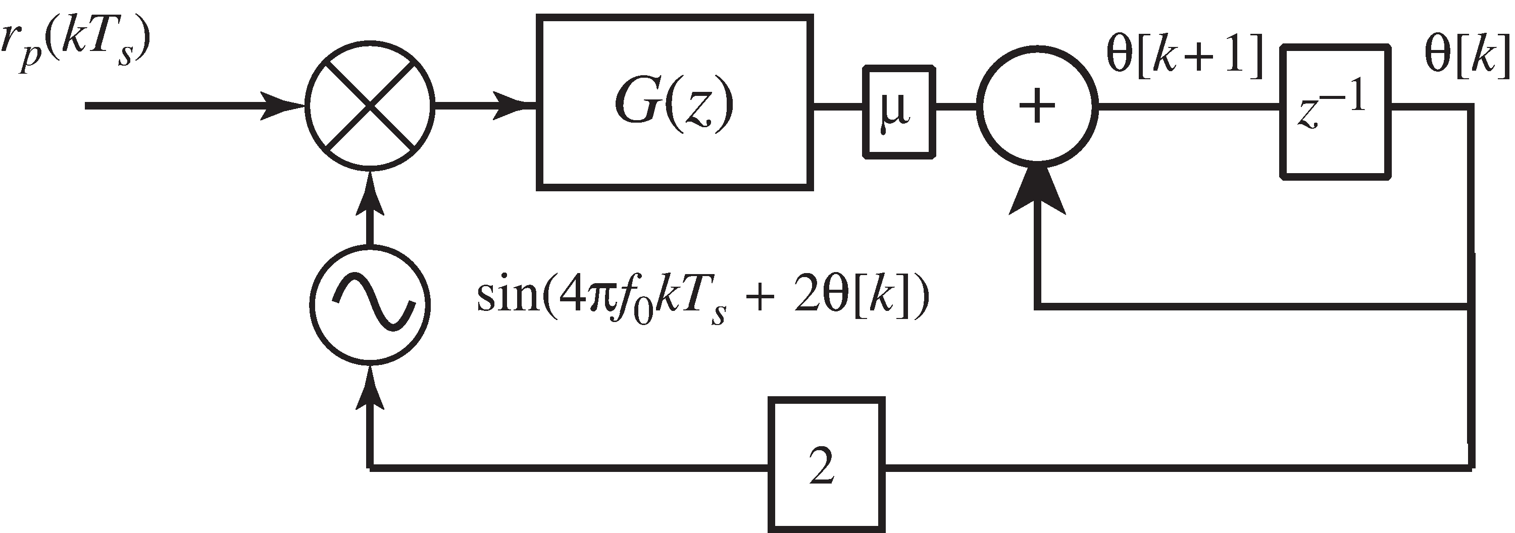
To see the operation of the generalized PLL concretely,
pllgeneral.m implements the
system of
[link] with
and
.
The implementation of the IIR filter follows the time domainmethod in
waystofiltIIR.m .
When the frequency offset is zero (when
f0=fc ),
theta converges to
phoff . When there is a frequency offset (as in the default
values with
f0=fc+0.1 ),
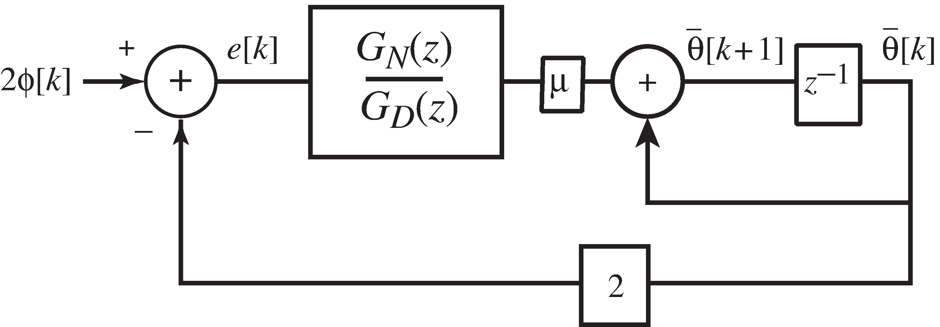
theta converges to a line. Essentially,
this
value converges to
in
the dual loop structure of
[link] .
Ts=1/10000; time=1; t=Ts:Ts:time;       % time vector
fc=1000; phoff=-0.8;                    % carrier freq. and phaserp=cos(4*pi*fc*t+2*phoff);              % simplified received signal
mu=.003;                                % algorithm stepsizea=[1 -1]; lena=length(a)-1;             % autoregressive coefficientsb=[-2 2-mu]; lenb=length(b);            % moving average coefficientsxvec=zeros(lena,1); evec=zeros(lenb,1);  % initial states in filter
f0=1000.1;                              % assumed freq. at receivertheta=zeros(1,length(t)); theta(1)=0;   % initialize vector for estimates
for k=1:length(t)-1                     % z contains past fl+1 inputs    e=rp(k)*sin(4*pi*f0*t(k)+2*theta(k));
    evec=[e;evec(1:end-1)];             % past values of inputs
    x=-a(2:end)*xvec+b*evec;            % output of filter    xvec=[x;xvec(1:end-1)];             % past values of outputs    theta(k+1)=theta(k)+mu*x;           % algorithm update
end

pllgeneral.m the PLL with an IIR LPF
(download file)
All of the PLL structures are nonlinear, which makes them hard to analyze exactly.One way to study the behavior of a nonlinear system is to replace nonlinear components with nearby linear elements.A linearization is only valid for a small range of values. For example, the nonlinear function is approximately for small values. This can be seen by looking at near the origin: it is approximately a line with slope one. As increases or decreases away from the origin, the approximation worsens.
The nonlinear components in a loop structure such as [link] are the oscillators and the mixers.Consider a non-ideal lowpass filter with impulse response that has a cutoff frequency below . The output of the is where represents convolution. With and , . Thus the linearization is
In words, applying a to is approximately the same as applying the to , at least for sufficiently small .
There are two ways to understand why the general PLL structure in [link] works, both of which involve linearization arguments.The first method linearizes [link] and applies the final value theorem for -transforms. The second method is toshow that a linearization of the generalized single-loop structure of [link] is the same as a linearization of the dual-loop method of [link] , at least for certain values of the parameters. [link] shows that for certain special cases, the two strategies (the dual-loop and the generalized single-loop)behave similarly in the sense that both have the same linearization.
What is the largest frequency offset that
pllgeneral.m can track?
How does
theta behave when the tracking fails?
Examine the effect of different filters in
pllgeneral.m .
pllgeneral.m has a lowpass character.a=[1 0] . What kind of IIR filter does this represent?
How does the loop behave for a frequency offset?b so that the loop fails?a and
b pair using
cheby1 or
cheby2 . Test whether the loop functions to track small
frequency offsets.Design the equivalent squared difference loop, combining the IIR structure
of
pllgeneral.m with the squared difference objective function
as in
pllsd.m .
Design the equivalent general Costas loop structure. Hint: replace the FIR LPFs in [link] with suitable IIR filters. Create a simulation to verify the operation of the method.
The code in
pllgeneral.m is simplified in the sense that
the received signal
rp contains just the unmodulated carrier.
Implement a more realistic scenario by combining
pulrecsig.m to include a binary message sequence,
pllpreprocess.m to create
rp , and
pllgeneral.m to recover the unknown
phase offset of the carrier. Demonstrate that the same systemcan track a frequency offset.
Investigate how the method performs when the received signal contains pulse shaped 4-PAM data.Verify that it can track both phase and frequency offsets.
This exercise outlines the steps needed to show the conditions under which the general PLL of [link] and the dual loop structure of [link] are the same (in the sense of having the same linearization).

Notification Switch
Would you like to follow the 'Software receiver design' conversation and receive update notifications?

|
|

|
|

|
|

|
|

|
|
|
|
|
|
|
|

|
|

|
|

|