

| << Chapter < Page | Chapter >> Page > |
Use Green’s theorem to calculate line integral
where C is a right triangle with vertices and oriented counterclockwise.
In the preceding two examples, the double integral in Green’s theorem was easier to calculate than the line integral, so we used the theorem to calculate the line integral. In the next example, the double integral is more difficult to calculate than the line integral, so we use Green’s theorem to translate a double integral into a line integral.
Calculate the area enclosed by ellipse ( [link] ).
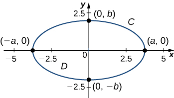
Let C denote the ellipse and let D be the region enclosed by C . Recall that ellipse C can be parameterized by
Calculating the area of D is equivalent to computing double integral To calculate this integral without Green’s theorem, we would need to divide D into two regions: the region above the x -axis and the region below. The area of the ellipse is
These two integrals are not straightforward to calculate (although when we know the value of the first integral, we know the value of the second by symmetry). Instead of trying to calculate them, we use Green’s theorem to transform into a line integral around the boundary C .
Consider vector field
Then, and and therefore Notice that F was chosen to have the property that Since this is the case, Green’s theorem transforms the line integral of F over C into the double integral of 1 over D .
By Green’s theorem,
Therefore, the area of the ellipse is
In [link] , we used vector field to find the area of any ellipse. The logic of the previous example can be extended to derive a formula for the area of any region D . Let D be any region with a boundary that is a simple closed curve C oriented counterclockwise. If then Therefore, by the same logic as in [link] ,
It’s worth noting that if is any vector field with then the logic of the previous paragraph works. So. [link] is not the only equation that uses a vector field’s mixed partials to get the area of a region.
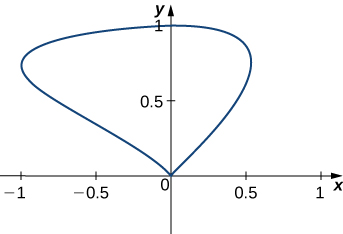
Find the area of the region enclosed by the curve with parameterization
The circulation form of Green’s theorem relates a double integral over region D to line integral where C is the boundary of D . The flux form of Green’s theorem relates a double integral over region D to the flux across boundary C . The flux of a fluid across a curve can be difficult to calculate using the flux line integral. This form of Green’s theorem allows us to translate a difficult flux integral into a double integral that is often easier to calculate.
Let D be an open, simply connected region with a boundary curve C that is a piecewise smooth, simple closed curve that is oriented counterclockwise ( [link] ). Let be a vector field with component functions that have continuous partial derivatives on an open region containing D . Then,
Notification Switch
Would you like to follow the 'Calculus volume 3' conversation and receive update notifications?

|
|

|
|

|
|

|
|

|
|

|
|

|
|

|
|

|
|
|
|