

| << Chapter < Page | Chapter >> Page > |
Quite often health professionals request that a patient a report their perception of their health status on a scale of 0 to 10, where 0 is the lowest possible health status and 10 is the highest health status. This type of data set is best analyzed using ordered probit. In this exercise you will analyze a data set of responses to a survey made in Germany between 1984 and 1995. The question we are interested in analyzing is the respondent’s perception of their own health status.
The file Riphahn, Wambach, Million data.xls is an MS Excel file that contains 27,326 observations on 25 variables, one observation per line. The data are from Riphahn, Wambach, and Million (2003) and are also available on the web . The variables are defined in Table 10. As a first step you will need to load these data into Stata. However, due to the large sample size you will need to first expand the size of the memory that is available to Stata with the command: . set memory 1G . Here I have increased the memory to 1 gigabyte. This amount may be overkill but it seemed to be big enough on my computer to handle the data.
| Column | Variable | Variable definition |
| A | ID | individual's ID number |
| B | Female | female = 1; male = 0 |
| C | Year | calendar year of the observation |
| D | Age | age in years |
| E | HSAT | health satisfaction, coded 0 (low) - 10 (high) |
| F | Handdum | handicapped = 1; otherwise = 0 |
| G | Handper | degree of handicap in percent (0 - 100) |
| H | HhnINC | household nominal monthly net income in German marks / 1000 |
| I | HHKIDS | children under age 16 in the household = 1; otherwise = 0 |
| J | Educ | years of schooling |
| K | Married | married = 1; otherwise = 0 |
| L | Haupts | highest schooling degree is Hauptschul degree = 1; otherwise = 0 |
| M | Reals | highest schooling degree is Realschul degree = 1; otherwise = 0 |
| N | FachHS | highest schooling degree is Polytechnical degree = 1; otherwise = 0 |
| O | Abitur | highest schooling degree is Abitur = 1; otherwise = 0 |
| P | Univ | highest schooling degree is university degree = 1; otherwise = 0 |
| Q | Working | employed = 1; otherwise = 0 |
| R | BlueC | blue collar employee = 1; otherwise = 0 |
| S | WhiteC | white collar employee = 1; otherwise = 0 |
| T | Self | self employed = 1; otherwise = 0 |
| U | Beamt | civil servant = 1; otherwise = 0 |
| V | DocVis | number of doctor visits in last three months |
| W | HospVis | number of hospital visits in last calendar year |
| X | Public | insured in public health insurance = 1; otherwise = 0 |
| Y | Addon | insured by add-on insurance = 1; otherwise = 0 |
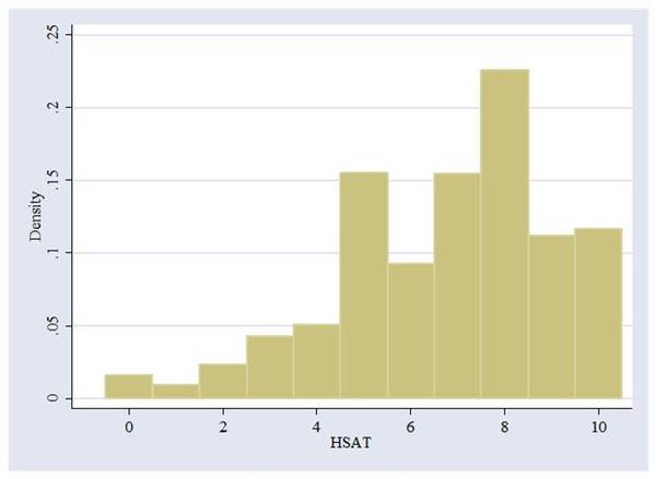
One of the major problems with survey indices is that the numbers seem to mean different things to respondents. One way to reduce this problem is to collapse the index into fewer outcomes by combining some of the responses together. However, anyway we do this is going to be ad hoc. Figure 6 shows a histogram of the responses to this question. Based on this graph, we will create 5 categories—(0) HSat = 0, 1, or 2; (1) HSat = 3, 4 or 5; (2) HSat = 6, 7, or 8; (3) HSat = 9; and (4) HSat = 10. We can create a new categorical variable called hsatnew with the command:
Notification Switch
Would you like to follow the 'Econometrics for honors students' conversation and receive update notifications?

|
|

|
|

|
|

|
|

|
|

|
|

|
|

|
|

|
|
|
|