6.1 Lab 6: analog-to-digital conversion, dtft and dft  (Page 2/4)

Quantization

Now change the Number of quantization levels for some fixed values of Frequency and Sampling Frequency. As the number of quantization levels is increased, the Digital waveform becomes smoother and a smaller amount of quantization error or noise is generated.

Signal reconstruction

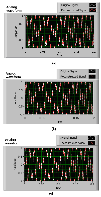
Next, set the frequency $f=\text{100}$ Hz and vary the sampling frequency. Observe the reconstructed waveform. [link] shows the reconstructed signals for three different values of skipped samples. If the sampling frequency is increased, fewer samples are skipped during the analog-to-digital conversion, which makes the reconstruction process more accurate.

Dtft and dft

In this example, let us compute and compare the DTFT and DFT of digital signals with the CTFT and FS of analog signals. [link] illustrates the completed block diagram of this transform comparison system. As discussed previously, to simulate an analog signal, consider a small time interval $(\text{dt}=0\text{.}\text{001})$ . The corresponding discrete signal is considered to be the same signal with a larger time interval $(\text{dt}1=0\text{.}\text{01})$ .

Generate a periodic square wave with the time period $T=0\text{.}1$ . Connect the input variable mode to an Enum Control to make the signal periodic or aperiodic. If the signal is periodic (case 0), compute the FS of the analog signal and the DFT of the digital signal using the fft function over one period of the signal. For aperiodic signals, only one period of the square wave is considered and the remaining portion is padded with zeros. For aperiodic signals, the transformations are CTFT (for analog signals) and DTFT (for digital signals), which are computed using the fft function. In fact, this function provides a computationally efficient implementation of the DFT transformation for periodic discrete-time signals. However, because simulated analog signals are actually discrete with a small time interval, this function is also used to compute the Fourier series for continuous-time signals. Because DFT requires periodicity, one needs to treat aperiodic signals as periodic with a period $T=\infty$ to apply this useful function. That is why the fft function is also used for aperiodic signals to compute CTFT and DTFT (as done in the earlier labs). However, in practice, it should be noted that the period of the zero padded signal is not infinite but assumed long enough to obtain a close approximation. Apply the same approach to the computation of CTFT and DTFT. Because DTFT is periodic in the frequency domain, for digital signals, repeat the frequency representation using the textual statement yd=repmat( yd,1,9) , noting that the fft function computes the transformation for one period only.