

| << Chapter < Page | Chapter >> Page > |
can make it run much more quickly. Specifically, in the inner loop of the algorithm where we apply value iteration, if instead of initializing valueiteration with , we initialize it with the solution found during the previous iteration of our algorithm, then that will provide value iteration witha much better initial starting point and make it converge more quickly.
So far, we've focused our attention on MDPs with a finite number of states. We now discuss algorithms for MDPs that may have an infinite number of states. For example, for a car,we might represent the state as , comprising its position ; orientation ; velocity in the and directions and ; and angular velocity . Hence, is an infinite set of states, because there is an infinite number of possible positionsand orientations for the car. Technically, is an orientation and so the range of is better written than ; but for our purposes, this distinction is not important. Similarly, the inverted pendulum you saw in PS4 has states , where is the angle of the pole. And, a helicopter flying in 3d space has states of the form , where here the roll , pitch , and yaw angles specify the 3d orientation of the helicopter.
In this section, we will consider settings where the state space is , and describe ways for solving such MDPs.
Perhaps the simplest way to solve a continuous-state MDP is to discretize thestate space, and then to use an algorithm like value iteration or policy iteration, as described previously.
For example, if we have 2d states , we can use a grid to discretize the state space:
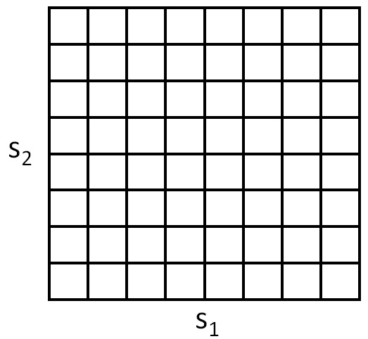
Here, each grid cell represents a separate discrete state . We can then approximate the continuous-state MDP via a discrete-state one , where is the set of discrete states, are our state transition probabilities over the discrete states, and so on. We can then use value iteration or policy iterationto solve for the and in the discrete state MDP . When our actual system is in some continuous-valued state and we need to pick an action to execute, we compute the corresponding discretized state , and execute action .
two downsides. First, it uses a fairly naive representation for (and ). Specifically, it assumes that the value function is takes a constant value over each of the discretization intervals(i.e., that the value function is piecewise constant in each of the gridcells).
To better understand the limitations of such a representation, consider a supervised learning problem of fitting a function to this dataset:
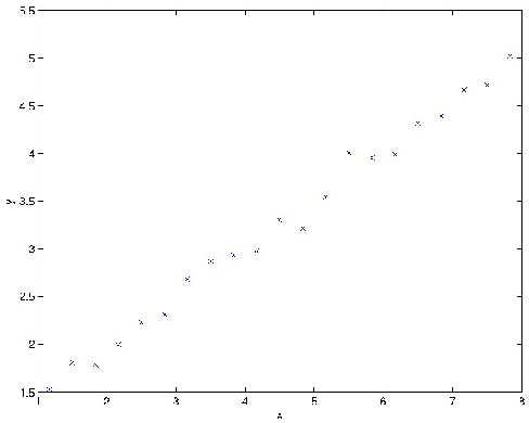
Clearly, linear regression would do fine on this problem. However, if we instead discretize the -axis, and then use a representation that is piecewise constant in eachof the discretization intervals, then our fit to the data would look like this:
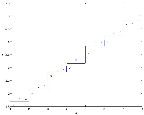
This piecewise constant representation just isn't a good representation for many smooth functions. It results in little smoothing over the inputs, and nogeneralization over the different grid cells. Using this sort of representation, we would also need a very fine discretization (very small grid cells) to get a good approximation.
Notification Switch
Would you like to follow the 'Machine learning' conversation and receive update notifications?

|
|

|
|

|
|

|
|

|
|

|
|

|
|

|
|

|
|

|