A distribution function determines the probability mass in each semiinfinite interval
. According to the discussion referred to above, this determines uniquely
the induced distribution.
The distribution function
F
X for a simple random variable is easily visualized. The
distribution consists of point mass
p
i at each point
t
i in the range. To the left of
the smallest value in the range,
; as
t increases to the smallest value
t
1 ,
remains constant at zero until it jumps by the amount
p
1 . .
remains constant
at
p
1 until
t increases to
t
2 , where it jumps by an amount
p
2 to the value
. This continues until the value of
reaches 1 at the largest value
t
n . The
graph of
F
X is thus a step function, continuous from the right, with a jump in the amount
p
i at the corresponding point
t
i in the range. A similar situation exists for a discrete-valued
random variable which may take on an infinity of values (e.g., the geometric distributionor the Poisson distribution considered below). In this case, there is always some probability
at points to the right of any
t
i , but this must become vanishingly small as
t increases,
since the total probability mass is one.
The procedure
ddbn may be used to plot the distributon function for a simple
random variable from a matrix
X of values and a corresponding matrix
of
probabilities.
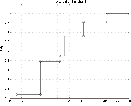
Graph of
F
X For a simple random variable
>>c = [10 18 10 3];             % Distribution for X in Example 6.5.1>>pm = minprob(0.1*[6 3 5]);>>canonic
 Enter row vector of coefficients  cEnter row vector of minterm probabilities  pm
Use row matrices X and PX for calculationsCall for XDBN to view the distribution>>ddbn                          % Circles show values at jumps
Enter row matrix of VALUES  XEnter row matrix of PROBABILITIES  PX
%  Printing details   See
[link]
We make repeated use of a number of common distributions which are used in many practical situations.
This collection includes several distributions which are studied in the chapter
"Random Variables and Probabilities" .
Indicator function .
.
The distribution function has a jump in the amount
q at
and an additional jump
of
p to the value 1 at
.
Simple random variable
(canonical form)
The distribution function is a step function, continuous from the right, with jump of
p
i at
(See
[link] for
[link] )
Binomial
. This random variable appears as the number of successes
in a sequence of
n Bernoulli trials with probability
p of success. In its simplest form
As pointed out in the study of Bernoulli sequences in the unit on Composite Trials,
two m-functions
ibinom and
cbinom are available for computing the individual and
cumulative binomial probabilities.
Geometric
There are two related distributions, both arising in the
study of continuing Bernoulli sequences. The first counts the number of failures
before the first success. This is sometimes called the “waiting time.” The event
consists of a sequence of
k failures, then a success. Thus
The second designates the component trial on which the first success occurs. The event
consists of
failures, then a success on the
k th component trial. We have
We say
X has the geometric distribution with parameter
, which we often designate by
geometric
. Now
or
. For this reason, it is
customary to refer to the distribution for the number of the trial for the first successby saying
geometric
. The probability of
k or more failures before
the first success is
. Also
This suggests that a Bernoulli sequence essentially "starts over" on each trial. If it has
failed
n times, the probability of failing an additional
k or more times before the next
success is the same as the initial probability of failing
k or more times before the first success.
The geometric distribution
A statistician is taking a random sample from a population in which two percent of the
members own a BMW automobile. She takes a sample of size 100. What is the probabilityof finding no BMW owners in the sample?
Solution
The sampling process may be viewed as a sequence of Bernoulli trials with probability
of success. The probability of
100 or more failures before the first success is
or about 1/7.5.
Negative binomial
.
X is the number of failures before the
m th
success. It is generally more convenient to work with
, the number of the
trial on which the
m th success occurs. An examination of the possible patterns and
elementary combinatorics show that
There are
successes in the first
trials, then a success. Each combination
has probability
. We have an m-function
nbinom to calculate these
probabilities.
A game of chance
A player throws a single six-sided die repeatedly. He scores if he throws a 1 or a 6. What
is the probability he scores five times in ten or fewer throws?
>> p = sum(nbinom(5,1/3,5:10))
p  =  0.2131
An
alternate solution is possible with the use of the
binomial distribution . The
m th
success comes not later than the
k th trial iff the number of successes in
k trials is
greater than or equal to
m .
Poisson
. This distribution is assumed in a wide variety
of applications.It appears as a counting variable for items arriving with exponential interarrival times (see
the relationship to the gamma distribution below). For large
n and small
p (which may not
be a value found in a table), the binomial distribution is approximately Poisson
.
Use of the generating function (see Transform Methods) shows the sum ofindependent Poisson random variables
is Poisson. The Poisson distribution is integer valued, with
Although Poisson probabilities are usually easier to calculate with scientific calculators
than binomial probabilities, the use of tables is often quite helpful. As in thecase of the binomial distribution, we have two m-functions for calculating Poisson
probabilities. These have advantages of speed and parameter range similar to those for ibinomand cbinom.
is calculated by
P = ipoisson(mu,k) , where
k is a row or
column vector of integers and the result
P is a row matrix of the probabilities.
is calculated by
P = cpoisson(mu,k) , where
k is a row
or column vector of integers and the result
P is a row matrix of the probabilities.
Poisson counting random variable
The number of messages arriving in a one minute period at a communications network junction
is a random variable
Poisson (130). What is the probability the number of
arrivals is greater than equal to 110, 120, 130, 140, 150, 160 ?
>> p = cpoisson(130,110:10:160)
p  =  0.9666  0.8209  0.5117  0.2011  0.0461  0.0060
The descriptions of these distributions, along with a number of other facts, are
summarized in the table DATA ON SOME COMMON DISTRIBUTIONS in
Appendix C .